PhantomNet
Attachments
-
 OpenEPC Sublicense Agreement
-
simeca-architecture
-
 Simeca architecture
-
simeca-prototype
-
MC-start
-
penb-log-attached
-
simeca-controller-log
-
simeca-p2p
-
enb-ho-log
-
SIMECA-controller-started
PhantomNet Main Wiki Page
Welcome to the PhantomNet Wiki!
EPC Components
- High-level / Administrative Documents
- Tutorials and Examples
- Reference Materials
- OpenEPC Documentation*
- Customizing OpenEPC Configuration
- OpenEPC frequently asked questions
Real Mobility Hardware
Off-the-shelf UE (Nexus 5) and eNodeB (ip.access e40) and SDR hardware now available for experimentation!
- Tutorials and Examples
- UE Interaction and scripting with Culebra
- Using SDR and OpenLTE in PhantomNet
- Combining Open Air Interface, SDR, and OpenEPC in PhantomNet
- Capturing and Dissecting RAN FAPI traces for the ip.access eNodeB
- Facebook App Example
- ACACIA mobile edge computing example
- SIMECA SDN-based mobile edge IoT example
- User-Contributed Content
- Reference Materials
Deprecated Tutorials/Examples for use with the "classic" PhantomNet interface
These remain only as a transitory reference for those who started with the NS-based experiment definitions. Please use the Profile-driven tutorials if at all possible.
Getting Help
OpenEPC General Information
Introduction
One of the key components available to PhantomNet users (who have agreed to the sub-license agreement) is the OpenEPC 3GPP framework implementation. Binary components are included on specially managed OpenEPC disk images. PhantomNet contains hooks to provision a collection of nodes into a functional OpenEPC instance. Each node runs one or more 3GPP components, as implemented by OpenEPC. PhantomNet assists users in setting up OpenEPC environments in two ways: First, it provides a template NS file that wraps many of the details of provisioning an OpenEPC instance. Second, backend scripts in the OpenEPC disk images take care of mixing OpenEPC setup into the traditional Emulab client-side, automatically bringing up components to create a fully functional OpenEPC instance.
Features
OpenEPC under PhantomNet provides the following:
- Flexible component provisioning
- EPC host access
- Mix in non-OpenEPC resources
- Emulate network conditions
Restrictions and Limitations
There are some restrictions and limitations related to PhantomNet's OpenEPC support.
- Restricted Binary-only OpenEPC images
- Topology limitations
OpenEPC Sublicense
Directly following this text is a link to the PhantomNet OpenEPC sub-license agreement. Please print, review, sign, scan and then email this agreement to phantomnet-approval@flux.utah.edu to obtain access to PhantomNet's OpenEPC-related materials. Be sure to note your PhantomNet username and project when submitting the agreement. Send questions or concerns about the agreement to this same email address.
If you would prefer to fax the agreement in:
- Flux Research Group fax number: +1 801 585-3743
- Attention to: PhantomNet Administrator
Motion modeling with PhantomNet attenuator matrix
Attenuator Code for Diverse Motion Modeling
Mark Van der Merwe
Report on internship project
Introduction
The PhantomNet project is dependent upon being able to create realistic motion models for the UE to follow. By creating these realistic models, we allow the user to test their applications during handover in ways more realistic to the outside world, while still maintaining the repeatable factor. In this way, PhantomNet can become a valuable asset to the mobile networking research community.
PhantomNet is designed to use attenuator boxes to simulate movement. By using these programmable attenuators, the system can accurately and repeatedly simulate movement.
The code documented here attempts to create three options which will allow people to easily test their applications on PhantomNet in several different ways. The options are:
- Testing individual attenuation points in a step-wise manner,
- Linear interpolation of attenuation points to create a more smooth realistic playback of recorded attenuations,
- Input of geometric locations for the UE rather than attenuations.
We believe these three options are a good start for creating useful motion modelling functions in PhantomNet.
Earlier versions of our work involved basic setting of attenuator values and learning the functionality of the attenuator device. Our early work also allowed us to test whether or not the attenuators behaved as expected. Our results were positive, though we are currently waiting for further equipment before more precise and accurate testing can take place.
Design
The code I developed was creating using Expect script, based on tcl. Expect allows us to automate interactive applications. We used its functionality to be able to enter commands into a command line to our attenuator. Expect gives us a lot of room to be smart and develop an interactive, smooth-working product.
Our code is designed to be run from an Emulab machine. This machine is connected through the Emulab network to the attenuator (via ethernet). SSH into the machine and you are ready to go. The code to start an Expect script is expect followed by the name of the file. For example to run this program we say: expect attenArray.exp. Note also that if you update the code in any way (change the attenuations, timestamps, heights, etc.) you will need to scp (secure copy) the file to the Emulab machine you are working on.
The attenuator used in our evaluation is a JFW MODEL 50BA-002-95 Benchtop Programmable Attenuator made by JFW Industries, Inc. It has two attenuators in it, each with an in and out port and a physical switch that can be used to change the attenuation manually. It is, as stated, programmable and we were able to use commands from the firmware manual to do what we needed with the code. Attenuator commands allow us to do many things with the attenuators but the two commands we took advantage of in this version are the set attenuator command, which allows us to set specific attenuations to specific attenuators, and the fade attenuator command, which allows us to fade between two attenuations for a specific attenuator. These two commands gave us the functionality we needed to create more realistic movement models.
Before detailing the functions, lets take a quick look at the first section of the code. (There are comments throughout the code for clarity as well). The first step of our code automatically telnets into the machine for us, giving us full access to all the commands provided by the attenuator. From there we set the attenuators to specific values: 0dB on attenuator 1 and -95 dB on attenuator 2. This just allows each test to start with the a similar environment, for repeatability’s sake. Next we lay out all the parameters for the specific functions. These parameters will be explained further on.
The last thing present before the code for the actual functions is a output to the user that is a small, basic description of the different options. Then we go into the interact loop which hands the process over to the user to decide which function to complete.
An example of the ouput in the beginning of the program.
As mentioned briefly in our introduction, our code contains three options for the users. Below is described the functionality of each in detail, the required user input parameters, and a brief description of the actual code behind the function. (With "user input parameters", we are referring to variables and arrays that we will eventually have the user provide. For now, these are simply defined at the start of the code)
Separate Points of Attenuation at Separate Times
As suggested by the name, this function takes an array of attenuation points and puts them into the attenuator with no interpolation. The array key is considered the timestamp for that attenuation. So the value at array(1) is the value the attenuator will show at time one. The array key will be considered the timestamp for all of the functions. The user must also input how long each timestamp is in seconds. So if a user says 3, then array(2) is really occurring at second 6.
The actual array does not have to be continuous. Users can input for times 1, 3, and 5 and the code will still work. A dictionary [2] is nested inside each key of the array and contains the attenuation values for all the attenuators allotted to the experiment. Our code is developed so that the amount of attenuators used is dynamic.
The actual code starts at 0 and increments up, stopping at each location that has an input value and sending that value to the attenuator. It then pauses so that we stay in line with the timestamps. If no value is given, the code simply pauses the time needed per step to simulate no change. It then continues incrementing and checking. Each time we find a value, we increment the number of successful updates we’ve completed. This number is then compared to the length of the inputed array to ensure we stop checking once we’ve reached the end of the array.
The output to the user is a time in seconds at each update to the system and the attenuation values for both of the attenuators. This lets the user easily track the progress of the system. Users should note that the system will pause if no update is asked and will say “Done.” when the process is completed.
Example of output to user and the done message.
Connected Points (Linear Interpolation) for a Given 'Path' of Attenuation Values
This function creates a more realistic path of attenuation. It takes an array of points, much like the one used in the first function, with each timestamp having an attenuation reading, and linearly interpolates between the points so that movement is more smooth and realistic. This function is especially created for people who have measured and recorded some movement in real life and want to “play it back” on the test bed.
User input for this is again an array with nested dictionaries. For this function, we are expecting that each timestamp has a value (starting at 0), so there are no gaps in time without updates. This is because we believe that it is a recording of sorts so the user will give us attenuations for each point. Keep in mind the points don’t have to be for every second since the user also inputs the time for each timestamp, much like in the above function (again timestamps 1 2 3 could really be seconds 3 6 9).
Our code again starts by finding how many values are given in the array. Next, we go through each part of the array, starting at zero, and going up till 1 before the last point. For each point, we find the attentuation (in dB) of that point and of the next one (thus why we stop one before the end). We then use the fade function, which allows us to increment automatically from one value to another every however many milliseconds. To find the amount of milliseconds, we take the time the user gave for each timestamp and multiply it by 1000 (gets it into milliseconds) and then divide it by the number of steps needed to be taken for that fade. This gives us all the values needed to fade between each point and the next. In this way we continue until we have reached the last attenuation.
Output includes the time at each update to the system in seconds. It also continuously displays the attenuation of both systems, allowing you to easily track the fade as it happens. When completed, the function will send “Done.” to the user. Note that for this function, the done may be followed by another output concerning the completion of a specific fade. This is because we cannot determine which attenuator will finish first, so we can’t specify what message to wait for. This should not have an effect on the overall timing however.
Example of output to the user and done message. Note the location of the done message (see above for details).
Motion Model Based on Geometric Inputs
The third function creates a different way for users to input data. If they don’t know the attenuation values they want but they want to be able to test movement around base stations, they can use this function. It allows them to use geometric inputs based on a basic (x,y) cartesian plane for the UE locations at different times. The function then finds the attenuations from these locations to the base stations, the location of which the user also determines, and thus simulates the wanted movements.
The first input from the user is an array with nested dictionaries that contains the geometric position of the UE. This position is made up of an x and y coordinate. These are measured in meters from a (0,0) origin (you can input negatives and decimals too). We again have a timestamp that dictates the timing of each point. We also don’t need points for every timestamp. For example, a user could say I want to be at (10,30) at time 0 and at (45, 20) at time 10 and the code would be able to use that and give back a accurate motion model between those points. Note however that the code is expecting a location for time 0. The user must also enter how long each timestamp is, just like the previous functions. Finally, the user must enter some variables to be used in the COST Hata Model (see below). These include UE and base station height (currently held constant for all base stations) and whether the experiment is in an urban or suburban environment.
Our code starts off by reorganizing the input. It takes the user supplied geometric data and puts it into a new array that places the timestamp as yet another dictionary value. This allows us to easily access the different points in a simpler matter later on. This also allows us to determine the total amount of updates to be done. In this function, we update several times a second (user inputs the number of updates per second too). Once we have the total number of updates to be done (time the user wants the experiment to run * updates per second), we start at update 0 in a for loop and go till the limit determined earlier. Each time we have a new update, we figure out between which two user provided geometric points this update lies and then use those two surrounding points to determine the exact location at that single update point. In the next step, the program takes the x and y location we just found and finds how far it is from each base station using the pythagorean theorem. These distances then independently plugged into the COST Hata Model [1]:
L = 46.3 + 33.9log(f) - 13.82log(hB) - a(hR) + [44.9 - 6.55log(hB)]log(d) + C
Where:
a(hR) = (1.1log(f) - 0.7)hR - (1.56log(f) - 0.8)
C = 0dB for medium cities and suburban areas
C = 3dB for metropolitan areas
L = Median path loss. Unit: decibel (dB)
f = Frequency of Transmission. Unit: megahertz (MHz). Must be between 150 and 2000 MHz.
hB = Base station antenna effective height. Unit: meter (m). Must be between 30 and 200 m.
d = Link distance. Unit: Kilometer (km). Should be between 1 and 20 km.
hR = Mobile station antenna effective height. Unit: meter (m). Must be between 1 and 10 m.
a(hR) = Mobile station antenna height correction factor as described in the Hata model for urban areas. (see above)
The model takes all these variable inputs and spits out an attenuation value (dB). Due to the high distance (between 1 and 20 km) we tend to get attenuations that are "higher" than we can set. We assume that the attenuator has about 40 dB insertion loss added onto every programmed value. For the final PhantomNet project, we will measure and incorporate this more precisely and we will consider tinkering with the base stations's power in order to emulate even higher attenuations. But for now we just assume 40 dB loss, so we subtract 40 dB from all the attenuations.
These we then plug into the set attenuator command. After that we pause for the amount of time indicated for each update. This we repeat until we reach the last given location. With this high speed updating, we allow a smooth, realistic motion model to be created based off of geometric values. One quick note, in order to allow for a cleaner output/execution, we only update the attenuator if the value to be sent to it changes.
The output for this function is, as before, a time in seconds followed by the respective attenuations. Again, when completed, the function will declare that it is “Done”. Also remember that the system pauses while waiting for the next input. Unless the done message has been set, the motion model is not yet completed.
Example of output to the user and done message.
Evaluation
In terms of testing these functions, there is not much we can do. Due to the fact that the PhantomNet project is waiting on some hardware, we cannot yet perform more precise and enlightening tests in terms of whether the attenuator does what we need it to do in terms of actually effecting the signal. So that means that for functions 1 and 2, we need to wait until we are ready with the new hardware. But for function 3, we needed to test to be sure that the math was correct and we were getting the right numbers.
Setup
In order to test this, we essentially inputed all the parameters needed and with a calculator, got the distance and attenuation in the same way the function does it. So using the pythagorean theorem, we found the distances for the values inputed. After doing that we used the Hata model to find the attenuation for those distances. Finally we went into the code and printed the distances and attenuations that the program found, so that we could compare them. You can still print out the distances and attenuations by uncommenting the two send_user lines in the third function. This will allow you to see the distance and attenuation for every potential update. If you'd like to see for the specific times we calculated, you will have to match up the update number to the second. This will depend upon the seconds per time slot and the rate of updates.
Below are the inputs I gave the system and the numbers I calculated separately (all locations are in meters from point (0,0)):
Base Station Locations:
Base station 1: x=0 y=1000
Base station 2: x=1000 y=3000
UE Height = 2 m
Base Station Height = 100 m (For both)
C = 0
Time = 3 seconds per timestamp
UE Locations:
Timestamp: x: y:
0: 0 1000
3: 67 1000
11: 245 1060
15: 335 1100
Distances:
UE timestamp 0 to Base 1: 1 km
UE timestamp 0 to Base 2: 2.236 km
UE timestamp 3 to Base 1: 1.002 km
UE timestamp 3 to Base 2: 2.206 km
UE timestamp 11 to Base 1: 1.087 km
UE timestamp 11 to Base 2: 2.081 km
UE timestamp 15 to Base 1: 1.149 km
UE timestamp 15 to Base 2: 2.013 km
Attenuation: (rounded to nearest whole number like in the program)
UE timestamp 0 to Base 1: 128 dB
UE timestamp 0 to Base 2: 139 dB
UE timestamp 3 to Base 1: 128 dB
UE timestamp 3 to Base 2: 139 dB
UE timestamp 11 to Base 1: 129 dB
UE timestamp 11 to Base 2: 138 dB
UE timestamp 15 to Base 1: 130 dB
UE timestamp 15 to Base 2: 138 dB
Results
Comparing these numbers we calculated separately to the ones that the system calculated, we ended up with the exact same answers for both distance and attenuation meaning the code is working as it should. This allows us to confidently say that the numbers being displayed by the program are accurate.
Conclusion
By using our expect script, we can emulate realistic movement for the PhantomNet project, giving users the ability to use our code in order to test and ensure their code works in real world situations. Our code is flexible to the user, allowing them several different options to choose from. The code allows the user to input separate attenuation points at separate timestamps, a linear interpolation of inputed points in order to play back attenuations, and a geometric input using function which allows the user to show us in a more physical manner what they want to test. This is a good start for creating an easy to use, realistic, highly repeatable testbed.
References:
- COST Hata model https://en.wikipedia.org/wiki/COST_Hata_model
- Dictionary Man Page (Tcl) http://wiki.tcl.tk/5042
Using OpenLTE and SDR hardware in PhantomNet
Introduction
PhantomNet supports software-defined RAN instances by combining software-defined radio (SDR) hardware and open source eNodeB software. We provide host PCs with USRP B210 RF hardware for the SDR hardware and OpenLTE is one of the supported eNodeB software implementations.
Hardware setup
The USRP hosts can be allocated with an NS file similar to the following:
set ns [new Simulator]

source tb_compat.tcl
set node [$ns node]

tb-fix-node $node nuc1

tb-set-node-os $node openlte-0-19
$ns run
The host is connected to the USRP via USB 3, and the connectivity can be verified from a shell on the host with a command like:
$ uhd_usrp_probe
This will also have the side effect of loading the USRP firmware if necessary.
To prepare the UE side of the RAN, you can operate one of the Nexus 5 handsets with an appropriate SIM card over the air (support for automatic allocation of UE devices and connectivity through the attenuator matrix is planned for the future). You will need to know the IMSI and IMEI of the UE.
eNodeB setup
To start the SDR eNodeB, you must first ensure the USRP firmware has been loaded (see above), and then start the OpenLTE eNodeB process on the host:
$ cd /usr/local/src/openlte-code/build/LTE_fdd_enodeb
$ ./LTE_fdd_enodeb
At this point, you should connect to TCP port 30000 on the host (with a telnet client or similar) to issue the configuration commands. You can optionally also connect to port 30001 to monitor debugging output. The eNodeB can be configured with settings like the following:
add_user imsi=xxxxxxxx imei=xxxxxxxx k=00112233445566778899aabbccddeeff
write band 4
write dl_earfcn 2175
write bandwidth 5
write tx_gain 30
write rx_gain 30
start
The IMSI and IMEI must correspond to the values programmed on the UE SIM card.
UE setup
Once the eNodeB is running, the UE should be able to locate the base station and receive PBCH messages. You should be able to connect to the LTE network, and send and receive IPv4 traffic through OpenLTE's emulated EPC.
Using commercial eNodeBs in PhantomNet
PhantomNet provides commercial eNodeBs for use by experimenters. Specifically, we currently have two ip.access e40 eNodeB devices available. (We expect to have more soon!) Each e40 is a dedicated LTE femtocell which can connect over the air to commodity UEs such as phones, tablets, or LTE modems. In most respects, they are self-configuring. They will automatically boot up and start talking to the OpenEPC infrastructure. We don't allow users to log onto these nodes directly. But we still provide an interface for changing some options and enabling logging information.
Creating your experiment
Before you can use an e40, you will have to add one to your experiment. You will need to add something like the below to your ns file:
# Add ip.access enodeb node #1
set penb1 [$ns node]
tb-fix-node $penb1 enodeb01
addtolan net_d $penb1
This creates a new node, specifies which e40 is uses, and adds that node to one of the management vlans.
Configuring Your eNodeB
The e40 must reboot each time you change the configuration. Because of this, the complete configuration (with defaults allowed) must be provided at once. Once you have created a configuration file (described below), you will need to use the e40-config.sh script:
e40-config.sh <ip> <configuration-file>
The script will contact the e40 at the given IP address and send it the specified configuration file. After the e40 changes the configuration, it will reboot to implement the changes. When the e40 reboots, all connections to both UEs and the MME will be terminated.
Configuration File
The configuration file consists of key/value pairs, one per line. Empty lines are permitted, and a line beginning with a '#' is ignored.
# Example Configuration File
# Here is a key/value pair
ReferenceSignalPower=-20
# All settings which are not explicitly specified are set to their default
The following keys are used for configuration:
- ReferenceSignalPower` -- This is the base power level in dbm used for broadcasting messages to the UE. Default: -10 Max: 5
A debugging interface called FAPI is provided for logging messages in the RAN. Enabling this interface is very resource-intensive and so may perturb the results of your experiment. When enabled, a tcpdump stream is sent to a specified address and port in real time which you can save or analyze. A proprietary parser, described elsewhere, must be used to analyze the stream.
- FAPI_IP -- The destination IP address for the tcpdump stream. Default: 0.0.0.0
- FAPI_Port -- The destination port for the tcpdump stream. Default: 8888
The following boolean flags indicate which messages on the RAN should be sent to the above IP and port. Set to '1' to enable:
- FAPI_PhyErrorInd -- Default: 0
- FAPI_PhyDlCfgReq -- Default: 0
- FAPI_PhyUlCfgReq -- Default: 0
- FAPI_PhyUlSfInd -- Default: 0
- FAPI_PhyDlHiDci0Req -- Default: 0
- FAPI_PhyDlTxReq -- Default: 0
- FAPI_PhyUlHarqInd -- Default: 0
- FAPI_PhyUlCrcInd -- Default: 0
- FAPI_PhyUlRxUlschInd -- Default: 0
Using the e40
Once you have configured your e40, it will automatically connect to the MME. You should see something like the following in your MME logs:
10(11032) 10:51:36 INFO:sctp_socket_accept():444> Notification 32769 to socket 13 received
14(11038) 10:51:36 INFO:mme_s1ap_recv_S1_SETUP_REQUEST():371> Received an S1AP Setup Request message
14(11038) 10:51:36 INFO:mme_s1ap_send_S1_SETUP_RESPONSE():281> Preparing the S1AP S1 Setup Response message
14(11038) 10:51:36 INFO:mme_s1ap_send_S1_SETUP_RESPONSE():345> Successfully sent the S1AP S1 Setup Response message
14(11038) 10:51:36 INFO:mme_s1ap_recv_S1_SETUP_REQUEST():432> Successfully processed the S1AP S1 Setup Request message
At this point, any UE with a key and IMSI in the MME's database can connect through the e40.
Rebooting
If you need to reboot the e40, simply reconfigure it and it will automatically reboot.
Questions
For any other questions, contact phantomnet-users@emulab.net
Dissecting RAN Messages using FAPI
Introduction
Our off-the-shelf eNodeB vendor, ip.access, provides a tool called FAPI that can be used to analyze RAN messages exchanged between the UE and the ip.access eNodeB in detail. The logs can be accessed as a tcpdump (pcap) trace and be analyzed by a custom Wireshark installation integrated with a FAPI plugin.
The verbosity level of the capture can be set according to the user preference. The default configuration allows a extremely verbose capture of all the RAN messages - e.g., RACH indications, UL/DL configuration requests, UL/DL scheduling information etc. An example capture is shown here. Such a verbose capture is very useful in understanding the overall message flow associated with different phases of device-network interaction including connection setup, data exchange, and connection teardown.
However, in certain scenarios a user may be interested in specific types of message exchanges - for example an user may want to focus only on RAN messages related to scheduling. ip.access provides filters that allow users to configure the FAPI logging to capture only the messages of interest and discard the others. The following table shows the set of options available to the user - one or more such options can be enabled in the eNodeB as per a user's configuration.
| enableFAPIPhyErrorIndLogging | Log only Error Messages |
| enableFAPIPhyDlCfgReqLogging | Log Downlink Configuration Request Messages |
| enableFAPIPhyUlCfgReqLogging | Log Uplink Configuartion Messages |
| enableFAPIPhyUlSfIndLogging | Log Uplink Subframe Indication Messages |
| enableFAPIPhyDlHiDci0ReqLogging | Log DCI-0 (Uplink Scheduling Assignment) Messgaes |
| enableFAPIPhyDlTxReqLogging | Log Downlink Data Transmission Request Messages |
| enableFAPIPhyUlHarqIndLogging | Log Uplink HARQ Indiaction Messages |
| enableFAPIPhyUlCrcIndLogging, | Log Uplink CRC Indication Messages |
| enableFAPIPhyUlRxUlschIndLogging | Log Uplink Scheduling Indication Messages |
| enableFAPIPhyUlRachIndLogging | Log RACH Indication Messages |
| enableFAPIPhyUlSRSIndLogging | Log SRS Indication Messages |
| enableFAPIPhyUlRxSrIndLogging | Log Scheduling Request Indicator Messages |
| enableFAPIPhyUlRxCqiIndLogging | Log Receiver Channel Quality Indication Messages |
| enableFAPIRFTickLogging | Log Clock Ticks |
For example, n user who wants to debug UL subframe indication messages can enable the "enableFAPIPhyUlSfIndLogging" option to get a trace like this. Similarly by enabling "enableFAPIPhyUlRxCqiIndLogging" the user can get detailed information about Channel Quality Indication report as can be seen in this trace.
In summary, FAPI is a great and powerful tool that enables an user to dive deep into the messages exchanged at the RAN. The flexible logging functionality is useful for both debugging specific types of messages and understanding the message flows and message contents in the RAN in general.
Accessing Pre-Captured Logs:
For the user's convenience we have captured FAPI logs, related to each of the aforesaid options, which can be accessed through a PhantomNet experiment. Once you have created a PhantomNet experiment, you can ssh into any of the experimental node to access the captured logs. The logs are located in /share/phantomnet/FAPI_caps/ directory. Each pcap file in this directory corresponds to a specific filtering option as described in the earlier section. We also have a fapi_all.pcap file that corresponds to the case when all the filtering options are enabled. Each capture corresponds to the following events: a) Device Attachment, b) Accessing a Internet-based webpage from the device, and c) Device Detachment.
Following is a step-by-step instructions as how you can access the pre-captured logs:
1. ssh -X sgw.[your experiment name].[your project name].emulab.net  (You can get your SGW's canonical hostname from the node list tab in your experiment as well.)

2. cd /share/phantomnet/FAPI_caps/

3. ls  <To list all the pre-captured files>

4. wireshark enableFAPIPhyDlCfgReqLogging.pcap <Open an example pcap to see its contents>
Generating Your Own Captures
Now we describe how you can capture your own FAPI logs using the configuartion options described in the Using commercial eNodeBs in PhantomNet guide. You can capture the logs using any physical node connected to the physical eNodeB in your setup. We recommend using the emulated eNodeB node [Ip address: 192.168.4.90] for this purpose. Following is an example guide that can be used to set the enableFAPIPhyDlCfgReqLogging at the eNodeB and capture the corresponding FAPI logs.
Step 1: Setup the eNodeB [Please refer to Using commercial eNodeBs in PhantomNet guide for details]
i) ssh into the SGW
ssh sgw.[your experiment name].[your project name].emulab.net
ii) create a config file test.cfg with the following options:
# Example Configuration File

# Specify capture node IP - we'll use the IP of the SGW node here.

FAPI_IP=192.168.4.80

# Specify capture port (we'll point tcpdump at this port)

FAPI_port=8888

# Specify FAPI option to enable.

FAPI_PhyDlCfgReq=1
iii) Configure the Physical eNodeB
e40-config.sh enodebXX test.cfg
In the above command, XX is a placeholder for the actual number portion in the name of the eNodeB in your experiment (e.g., enodeb03). You should be able to find this canonical name by looking for the eNodeB in the List View tab for your experiment on the PhantomNet web portal. This configuration command will reboot the eNodeB and set it up with the required logging capabilities.
Step 2: Capturing the FAPI logs
i) Figure out which interface to capture from. The eNodeB nodes all connect via the net_d subnet (192.168.4.0/24). The following command will show you the net_d interface of the SGW node:
ip address show to 192.168.4.80
ii) Execute tcpdump to capture FAPI logs on your SGW node (save to local disk by changing to /var/tmp):
cd /var/tmp
sudo tcpdump -i [interface found in prior command] -s0 -w my-FAPI.pcap port 8888
Here 8888 is the port we set for the eNodeB to log to in the configuration file we created above.
Once this capture is enabled, you can use your UE device to connect to the eNodeB and access the Internet. Once you are done with the experiment, you can use [Ctrl C] to stop the tcpdump capture and use wireshark to access the captured log.
FAPI_files
-
fapi_ulsfi
- UL subframe indication
-
fapi_cqi
- Channel Quality Indicator trace
-
FAPI_all
- default FAPI capture
Facebook status update tutorial using PhantomNet portal
Overview
This tutorial will walk you through the steps to build and install test Android applications that control a Facebook application to do certain tasks programmably.
In particular, Alice uploads a photo to Facebook every 3 minutes for 10 times and Bob (a friend of Alice on Facebook) continuously updates for the photos. We measure the time to complete a post and the time for a photo to be fetched from Facebook servers.
This functionality might be useful for users who want to understand how real applications function under various network conditions, or how mobile network protocol changes impact a smartphone application.
This tutorial will be done in the PhantomNet (https://www.phantomnet.org) testbed via PhantomNet portal and geni-lib, using two Nexus 7 tablets attached to an Ip.access E-40 small cell and a OPEN EPC core network instant.
Git repository
The tutorial is packaged in a Git repository. Clone the repository:
git clone git@gitlab.flux.utah.edu:binh/android-sdk-facebook.git && cd android-sdk-facebook
The cloned folder consists of 3 sub-folders:
- apk: includes Facebook apks and scripts to re-sign the apk.
- scripts: includes the scripts for the tutorial.
- test-blackbox: includes Java source code of the test applications.
Create a profile and initiate an experiment using PhantomNet portal and Geni-lib
1. Topology overview:
Figure 1 shows the topology of the experiment in PhantomNet.
In the radio side of the network, two Nexus 7 tablets running Android 4.4.2 are attached to a Ip.Access (E-40) LTE small cell base station via LTE.
In the core side of the network, an OpenEPC instance consists of EPC components needed for a LTE/ECP network (i.e, SGW, MME, PGW, HSS). PGW is the gateway connecting the core network to the Internet (and Facebook servers).

Figure 1. Tutorial topology
2. Create experiment profile in PhantomNet portal using Geni-lib:
PhantomNet allows users to create a profile that specifies topology, parameters, and set up scripts. After having a profile, multiple experiements could be initiated using the profile, each experiment will be an instance of the profile. In this tutorial, we will create a profile using Geni-lib source code in PhantomNet portal.
Step 1: Go to PhantomNet website at https://phantomnet.org and log in.
Step 2: In your personal homepage, create a profile by select "Create Profile" under "Actions".

step 3: Assign a name for your profile. Then click on "Source" next to "Topology" button to specify the profile using a Geni-lib script.

step 4: Upload a Geni-lib Python script to specify the topology of the profile. Here is the geni-lib script that specifies the topology for our tutorial. Copy and paste the geni-lib script and click "Upload". Click "Accept" to finish uploading.
step 5: After uploading the geni-lib script, an Rspec will be generated for your profile. The Rspec specifies the resources (e.g., nodes, links) in an XML format. To see how the RSpec looks like, click on "XML" button in the "Create Profile" page (note that the XML is read-only, if you want to modify the topology, you would need to modify the geni-lib script).

2. Instantiate an experiment in PhantomNet using the created profile:
Now as you created a profile that specifies the tology for your experiment, you can instantiate an experiment using the profile:
Step 1: To select the profile you have created, click on "Actions"->"My Profiles". Click on the profile that you created.

Step 2: Instatiate an experiment by click on "Instantiate" button. Click "Next" in the Select Profile page. Click "Next" in the Paramiterize page. Put a name for your experiment in the Finalize page and then click "Finish".

Step 3: After clicking "Finish" it might take up to 10 minutes for your experiment to be created and ready. You can see your experiment being instantiated on the flight. Once the experiment is ready, click on "List View" for ssh information of how to access your nodes.

Resign the Facebook apk
In order to let other apks control the Facebook apk, we need to resign the Facebook apk using a development key. We use zipalign to sign the Facebook application. On your computer install "zipalign" by:
sudo apt-get install zipalign
In this tutorial we use Facebook 25.0.0.19.30. The original apk could be found in apk/Facebook- 25.0.0.19.30.apk
Since we need to control the Facebook apk without knowing the source code of it, we need to re-sign the apk using a debugger key. While you can use any key to re-sign the apk, we will use Android's default debugger key that comes with the standard SDK to sign the apk:
bash apk/signapk.sh apk/Facebook-25.0.0.19.30.apk apk/debug.keystore android androiddebugkey
After this step, a re-signed apk will be created in the apk folder named apk/signed_Facebook- 25.0.0.19.30.apk. We’ll use this apk throughout this tutorial.
Install the resigned Facebook apk to the Nexus 5 devices:
We need to install the resigned Facebook apk to the 2 Nexus 5. We will use "adb" interface to do this.
First, we tell PhantomNet to connect to ADB daemon on the Nexus 5 via a special ADB target by:
$> pnadb -a
List the available devices in the experiment by:
$> adb devices
List of devices attached
0fabdc5e device
1fab7f8a device
Install the apk to the devices using the device IDs above:
adb -s 0fabdc5e install apk/signed_Facebook-25.0.0.19.30.apk
adb -s 1fab7f8a install apk/signed_Facebook-25.0.0.19.30.apk
The test applications
We need two test applications for Alice and Bob that launch and control Facebook apk to do predefined tasks: Alice uploads a photo to Facebook and Bob continuously fetches the photo.
The two applications are Android test applications and their apk could be found in apk/alice.apk and apk/bob.apk.
Note: If you would like to see how the apks were implemented, please refer to test-blackbox folder. In short, Alice opens the Facebook apk, touches on update status button and post a photo every 3 minutes for 10 times; Bob opens Facebook apk, scrolls down the main feed screen to fetch new updates from Alice.
During execution, Alice measures the time to post a photo (i.e, the elapsed time between touching the post button and the moment the progress bar disappears); Bob records the moment that photo appears on Bob’s main feed. The fetching time is the elapsed time between the moment the photo was posted by Alice and the moment it appears on Bob’s screen.
The source code for Alice and Bob apk are in "/test-blackbox/alice/src/com/testAlice/" and "/test-blackbox/bob/src/com/testBob/".
Install Alice and Bob apk applications to the Nexus 5 devices:
We need two test applications for Alice and Bob that launch and control Facebook apk to do predefined tasks: Alice uploads a photo to Facebook and Bob continuously fetches the photo.
The two applications are Android test applications and their apk could be found in apk/alice.apk and apk/bob.apk. To install the two applications:
adb -s 0fabdc5e install apk/alice.apk
adb -s 1fab7f8a install apk/bob.apk
Sign up for Facebook accounts and log-in manually:
The tutorial assumes you already logged into the Facebook accounts on the Nexus 5 devices so that the scripts will post Facebook status automatically without the log-in actions. Therefore, you will need to create 2 Facebook accounts manually (e.g., using your own computer and the Facebook website). The accounts could have any name as you wish. After having the account, log-in to Facebook accounts on the Nexus devices. A way to log-in to Facebook is via a GUI interaction with the devices using Culebra. A tutorial of how to use Culebra to interact with Nexus 5 via GUI is here.
Run the test applications and observe:
Finally, we need to run the Alice and Bob Apps. The apps will execute the auto-post and auto-fetch actions on Facebook. There is a script to wakeup and unlock the devices and launch the Alice and Bob apks:
bash scripts/alice-bob.sh
During the execution of this script, if you have a Culebra GUI window open, you will see the Alice and Bob apks control the Facebook apk to post/fetch status.
Gathering results
After running the test applications, two log files are created inside the scripts folder: scripts/alice.logcat and scripts/bob.logcat. alice.logcat records the moment Alice clicks on the post status button and the moment the photo is posted. bob.logcat records the moment the photo appears on Bob’s screen. Note that each photo is posted with a unique hash text that is used to distinguish them to calculate elapsed time. You can open the logcat files (i.e., using "adb shell") and calculate the elapsed time yourself or use the following script:
bash scripts/process_delta_time.sh
The output of this script is status|post time|fetch time, where post time is the elapsed time to post a photo on Alice in millisecond and fetch time is the time for Bob to fetch the photo in millisecond.
Conclusions
This tutorial showed you the steps to run test applications to control Facebook apk and observe the interactions between Facebook and a LTE/EPC network. Similarly, you can build your own test applications to control other apk such as Youtube, Twitter to understand how the apps interact with the LTE/EPC network or how the LTE/EPC network performance could affect the apps.
Tutorial: Interacting and Scripting on the UE with Culebra
Introduction
The PhantomNet testbed is designed to allow users to emulate realistic networks using the emulab system. In order to make this testbed useful to developers, we must then develop an interface that allows users to interact with the UE devices provided on the PhantomNet infrastructure as well as develop scripts to automate tests. We use the Culebra GUI, built on AndroidViewClient, to allow this functionality. This tutorial will take you through the process of interacting with the UE device on the PhantomNet testbed as well as scripting on it. We will also cover using Culebra on your local machine in order to create a test on a phone hooked to your machine and then sending and running that test script on the remote device.
Interacting Manually with the UE
Instantiate a PhantomNet experiment: Go to PhantomNet’s website. In the top right corner, hit Log In and enter you username and password. This will take you to the screen to instantiate a PhantomNet experiment (If it doesn’t, click on Actions on the top left and then on Start Experiment). Here, click the choose profile button and select OTS-Hardware-RAN. Then click Select Profile in the bottom right. A brief description of the topography appears. In the bottom right, click the Next button.

In the second screen, leave the parameters as their defaults and click Next.

This will take you to the final screen. Here you can enter a name for the test (optional) and get a closer look at your setup before you start the experiment.

Finally, click Finish. This will begin the setup of your PhantomNet experiment.

What we just created is a virtual network, the network core being OpenEPC software running on three nodes (SGW, PGW, and EPC nodes). This core is then connected to the EnodeB, which is an actual physical EnodeB present in the setup of the experiment. These act as the base stations. Then, we have a real UE device (Android phone, in our case, a Nexus 5). This is connect to the base station, and our attenuator matrix between the two will allow us to tinker with the network. The final node allocated in the experiment is the adb-tgt node. This node is put mostly for ease of use. On this node, we preload all the tools necessary to interact and script on the UE. We will go into more detail later on into the specific functionalities provided. We will work out of this node to run culebra and adb commands (will provide more details later).

While the experiment is being set up, we will need to insure that you will be able to connect to and see what the adb-tgt node sees. In order for this to occur, make sure you have both added your ssh key to the PhantomNet's site and installed and X11 forwarding system. These in combination will allow us to see what the adb-tgt node is seeing. In order to add your ssh key, go to Actions in the top left and hit Manage SSH Keys. If you ever need to find your way back to your experiment, you can always hit Actions and then My Experiments. From there you can reopen your experiment's page. If you don't have an X11 forwarding system, follow the corresponding instructions below, otherwise skip ahead to the next instruction.
MacOSX: Mac uses a program called XQuartz to allow X11 forwarding. To download, go to XQuartz's website, download the .dmg, and follow the installation instructions. Once you have this completed, XQuartz will be added into your utilities folder in Applications. Open the program, and when you see it's name in the menu bar, click Applications, then Terminal. This will open an Xterm terminal. Use this terminal to complete the next steps.
Windows: Windows uses a program called XMing. To download use the XMing site. Go to the files tab, then to the XMing folder and download the setup executable. Once this is installed, you should be able to start up your X server by going to all Programs and running XMing. More details on usage can be found at the XMing site.
Linux: Linux requires no installations, only the -Y in the ssh call. As this is specified in the future instructions, Linux users can skip to the next instruction.
NOTE: This tutorial was created on a Mac, so be warned that Windows and Linux instructions maybe require some additional work (XMing in particular) on the part of the user. Be sure to read through links to ensure your system is up to scratch for your system version.
Once the experiment is all setup and you have X11 forwarding setup, go to your X server terminal. Then, on your experiment page, click on the List View tab, and find the row for the adb-tgt node. Next type the following into your x-terminal, substituting your PhantomNet username and the Node Name for adb-tgt specified in the list view:
ssh -Y username@node_name.emulab.net
For example:
ssh -Y bob@pc999.emulab.net
This will ssh you into the node, and set up the X11 forwarding with the -Y option.
Once inside, you will use ADB to interact with the phone. ADB stands for android debug bridge, and is a system created by Android to allow control and interaction with the phone through the command line. In order to connect to the UE device, we can use a wrapped version of ADB. In the command line, type:
pnadb -l
This will list the UEs available, in our case, the single UE device we instantiated in the profile.
UE Nodes
Name Node ID Console Server Port
------------------------------------------------------------------------------
rue1 ue1 pc599.emulab.net 8001
As you can see, we connect to our UE through a port on pc599.emulab.net, which in this case is 8001. In order to connect through adb to the device, you can either follow the prompt, or do the easy:
pnadb -a
This will start up the adb daemon and connect to all available devices.
* daemon not running. starting it now on port 5037 *
* daemon started successfully *
connected to pc599.emulab.net:8001
If you have modified the profile and would like to only connect to one, you could run (substituting in your port number):
adb connect pc599.emulab.net:port_number
If you would like to explore more with adb, you can view more possible actions here. We will not revisit ADB seriously in the remainder of this tutorial, however, it can be used to access the phone's shell, run and exit programs, and install and uninstall apks.
Once we're connected, we can use the Culebra GUI system to see and interact with the phone manually. Culebra is a python-based system that allows you to connect to, view, and interact with a device connect to a machine over ADB. More about Culebra GUI here. Run:
culebra -s pc599.emulab.net:port_number -uG -P 0.25
This will open up a separate window on your screen. Give it time to load, until it says Culebra and then a version number on top.
- If your system throws an error that looks like the one below, it means your X11 forwarding system is having trouble setting up and should be revisited.

Once the screen loads, there is a good chance the screen will be black, as the UE is asleep. To solve this issue, right click on the screen and select Wake Up or click Ctrl-K to open the control panel, hit Power in the top right, then click back on the phone screen and click F5 to refresh the image (you can do it at any time to refresh the image from the phone).

Once you've woken up the phone, you can now play around with the GUI. You can click on the screen, and it will tell you to wait, and then load the following screen. IMPORTANT: This system works great, but relatively slowly. Be patient and only complete one action at a time.

Some points about our usage of Culebra:
- We use -s pc599.emulab.net:port_numberI so that Culebra can find our device using its serial number.
- We use -G to open the GUI.
- The -u tells the system not to take a full snapshot of the phone screen and inspect it's items. We turn it off during interactions in order to speed up the speed of the system. We will further discuss its usage later during the scripting portion of the turorial.
- The -P 0.25 scales the phone image down on the screen. Because it does a pixel to pixel approximation, and the phone has a higher pixel density, we must scale down or the screen is giant. Feel free to change this for your screen's resolution.
Some tips for interacting with the Culebra GUI:
- You can always press F5 to refresh the image on the screen.
- Typing Ctrl-K pulls up the control panel which provides additional buttons and options, as well as a keyboard.
- In order to drag, right click and then choose Drag Dialog. Then click grab next to starting point and click where on the screen you want the drag to start. Next, click grab next to the end point and click where on the screen you want the drag to end. Then, click Ok. The page will refresh, with your drag complete.
Scripting with the Culebra GUI on the Remote Device
You may have noticed that in the terminal we called the culebra command from, a script is generated. As we click around the GUI, the script is automatically generated by the Culebra system. That script can be played back to repeat the actions we just completed in the GUI. In order to save it to a file we can playback, we need to adjust the way we are calling the culebra command.
- To start, we need to add the -U tag. This tag tells the system to generate a Unit test and is required for the script to play back correctly.
- The next thing we need to do is add the -o tag. By adding this followed by a file path, we tell the system where to store the script. Generally, we store in the user's home directory: ~/filename.py. When we add this option, we will no longer see the script being created in the terminal.
- Before we run the new script, we should revisit and reexamine the -u tag. Culebra as a service automatically captures each screen and take what they call a dump, that is, they see what's on the screen and record it in the script. That way, when we go back and play the script, if everything isn't as expected, the test will fail. This can be useful if you would like the test to confirm the state of the phone before taking the next step. If this is not a concern, you can add the -u back in, and we will only look for the button pressed, instead of back checking the entire page. Because we are writing the script on the same phone we will run it back on, our trials so far show that -u makes the system a little easier and faster to use but if you need that verification, you can always remove the -u and get the screen state after every step.
- Another thing we can consider adding is the -L tag. This tag logs the actions of the script to the adb log. This means if you read the logcat later, the actions, like click on settings, will appear in the output. We will not add this for the example illustrated here, but if we are to run a test on our own application, this could be more useful.
As an example, run the script below, noticing the tags we have added.
culebra -s pc599.emulab.net:port_number -uUG -P 0.25 -o ~/myfirsttest.py
Then click on the settings button and wait for the page to load.


Then click the Display button. Finally, click on the sleep button, and choose Sleep after 30 minutes of inactivity.


When you are finished, click the close button on the culebra screen. This ends the script generation. Again, you may need to be patient with the system as it tends to react slowly. Now when we run ls in the home directory we see myfirststep.py.
Before running the script you must insure that you are on the same page that you started the test script in. So if I start the script from the home screen, run the script from the home screen. If we do not run from the same screen even with screen dumping off, the system will give an error similar to the one below.

If you see an error similar to this one above, make sure you are on the same page you started your test on (this applies to a test with/without the -u). In order to take it back to the home screen, you can type in this shortcut to take care of it for you:
adb shell am start -a android.intent.action.MAIN -c android.intent.category.HOME
When you are ready to run the script:
./myfirststep.py -s pc599.emulab.net:port_number
After you run the script, a success should output something like this:

Once this is done, you can confirm the results of the script by opening the culebra screen again (without saving the script, since we're just checking that our script worked):
culebra -s pc599.emulab.net:port_number -uG -P 0.25
Adding -v when we run the script will make the output more talkative, so it will tell you what it is both clicking on and checking for as it goes through the script.
Feel free to go back through and play with the settings and setup of both the scripting and the running of the script. As always, you can add --help after each to see the options you have.
Scripting with the Culebra GUI using a Local UE
In developing the interface for our users, we realized a potential option for ease of use would be if the user could hook a phone up to their local machine, and run the resulting tests on the remote UE.
To start, we must make sure that ADB is installed on your local machine and is functioning. Note, ADB/Android tools require updated Java.
Linux:
sudo apt-get install android-tools-adb
For Mac and Windows, you will probably have to install the entire SDK:
Mac: Install from android-sdk_r24.4.1-macosx.zip.
Windows: Install from installer_r24.4.1-windows.exe.
Before moving on, check that your ADB is functioning as it should be. Connect an android phone to your local machine via USB connection. On the phone, navigate to settings and scroll down to developer options.

Inside developer options, make sure USB debugging is enabled, otherwise, ADB won't be able to connect to your device.

If you don't see developer options, go to About Phone at the bottom of the Settings page, scroll down to Build Number, and click it 7 times. This will enable developer options on your phone.
Once you've done this, go back to your terminal and type:
adb devices
Much like the wrapped version we used on the adb-tgt node in our experiment, it will start the ADB daemon and connect automatically to your device. You should see an output similar to the one below:

Once you are connected you can play around with your phone much like you were able to when you were connected to the UE on the adb-tgt node. ADB also allows us to connect to the device using the Culebra GUI.
Next, we must download the Culebra software onto your local machine. In order for the GUI to work, you must download the latest version of Python 2.x. Do not download Python 3.x as the Culebra system is designed to work with Python 2.x. Follow the instructions to update python and add the necessary Pillow add-on.
Open this page, and then open a terminal and write:
python -V
This will print out your Python version number. Check this number with the one on the top of the downloads page (the 2.x number) you just opened in your browser. If they are the same, you're good to go, otherwise download the newer version. Follow the download instructions, then run the above command again to make sure you have the new version installed.
To download AndroidViewClient (Culebra's "Parent") and Pillow (window system for python) complete the following steps:
Linux:
sudo apt-get install python-setuptools
sudo easy_install --upgrade androidviewclient
This downloads the AndroidViewClient. Then for Pillow:
easy_install Pillow
MacOSX and Windows:
For Mac and Windows we recommend using the pip tool from python:
pip install -U setuptools
sudo easy_install --upgrade androidviewclient
This downloads the AndroidViewClient. Then for Pillow:
easy_install Pillow
Now we should have all the pieces in place to start using the Culebra GUI on the local device. Make sure your device is connected over ADB the type:
culebra -uG -P 0.25
Note that we no longer spell out the serial number. Due to our PhantomNet infrastructure, we have to manually pass the serial number, but when using Culebra on your local machine, this is not necessary (unless it can't find the device in which case go ahead and add it). This command will open up a pillow window that will, like before, be the view of the screen. We interact with it in the exact same way that we interacted with the one we generated from our X forwarding. Like before, we can also add the -o followed by the filename and the -U to generate a script we can play back.
However, because we are no longer using the same device, we have complications. Because the screen on your local phone is most likely different from the UE device on PhantomNet, adding the -u is most likely necessary so that it doesn't crash due to the difference in phone screens. Adding the -u solves this problem given you are using the same android version. If you are not we run into some more complications, ones that we can solve by looking closer at the way the Culebra system generates its scripts.
The system is built on identifying views, and then subsequently interacting with them. Even if we add the -u (reminder: with this option, it no longer confirms the state of every screen) it still tries to identify the buttons on the screen we are clicking when generating the scripts. The system completes this by using three different recognizing attributes:
- findViewById() - uses a generated ID for the view (button) on the screen to identify and find the one you are interacting with.
- findViewWithText() - uses the text for the view to identify and find the one you are interacting with.
- findViewsWithContentDescription() - uses the description of the view to identify and find the one you are interacting with.
When scripting across a version difference (our UEs on PhantomNet are currently Android 4, while many Androids are now Android 5), you may find an error similar to this:

Looking through the error message, we see that our attempt to run the script has failed because: Couldn't find View with content-desc='Settings'. The script I ran to generate this error was created on a device with Android 5 before being run on our Android 4 device in PhantomNet. As we can see it is the third way of finding and identifying the views that is causing our script to crash. If you develop a script and see this kind of error, first check that you are starting on the same page you started the script from. If the error is still occurring like above, we can remove several of the three ways the system finds the views. By adding -option off to our call of culebra, it will no longer use the option specified.
Remove Find View by Id add: -i off
Remove Find View by Text add: -t off
Remove Find View by Description add: -d off
By playing around with these settings, you should still be able to generate a script on a different version of Android and play it back on our Android 4 UE device. If you can't get this to work, you can always use our adb-tgt to generate the script, like we did earlier.
Something to notice, is that when you don't click on a button, for example, if you click somewhere in open space, the system uses pixels to identify where you clicked. Thus if you have a different pixel density and click somewhere that is not a button, that click might end up somewhere else on the remote UE device. This is something to consider when creating your script.
To test that you can effectively create a script locally and run it on the remote, we will attempt to replicate the script we created on the remote but on the local. To start, make sure the phone you have hooked to your machine has the settings app on its home screen. This means you can interact similarly to the remote UE. When you're ready, type into your local machine terminal (substituting in your file path to save the script):
culebra -uUG -P 0.25 -o /Path/To/File.py
As before, click on the Settings app, then go to Display, then on Sleep, and set the Sleep setting to 5 minutes this time (This will allow us to see the change on the remote when we run the script). When you have completed this, once again, click on the x in the top left corner of the screen, and you should see the python script wherever you told the computer to save it. Next, we will copy this script over to the adb-tgt, where we can then run it on the remote UE. To do this
scp /Path/To/File.py username@pchost.emulab.net:~/filename.py
Substitute in your path to the local test file, your username, your pchost (get this from the list view of your PhantomNet experiment), and finally the filename you want the script to be saved to on the remote. Once you've done this an ls on the adb-tgt will show your file. Once again, make sure the phone is on the correct starting page and run the script:
./filename.py -s pc599.emulab.net:port_number
As before, the test should run, send a success message, and you can open a culebra connection to make sure it worked!
Interacting with hardware UEs
Introduction
Working with hardware UE devices in PhantomNet is a bit different from developing locally. Normally when developing with an Android device, you would plug the device into the USB port of your local computer and interact with it using tools such as ADB. Since the UE devices in PhantomNet are in a remote location, the PhantomNet testbed sets up remote access. With a few minor adjustments, you should be able to work with the UE devices in PhantomNet just as you would with local devices attached to your computer.
How UE access is setup
You must specify to PhantomNet that you plan to interface with your hardware UEs. If you don't, the UEs will still be allocated, and will attach to your EPC, but you won't be able to interact with them via ADB, etc. The system-provided PhantomNet profiles that request UE hardware also request out-of-band access to be setup for these devices. See for example the following profile:
Off The Shelf Hardware Radio Access Network profile
These profiles request a dedicated ADB target node, and set an attribute on any UE nodes in the profile script to point them at this node. When an experiment is instantiated from such a profile, the PhantomNet setup machinery forwards a connection from the adbd daemon running on the UE through the infrastructure host it is connected to (via USB). It only allows the ADB target node to connect to this forwarded connection. In other words, the infrastructure host connected to the UE listens on a dynamic TCP port for connections from an ADB target, and forwards this traffic on to the adbd daemon running on the device. The ADB target node is further setup to load and run a disk image that contains tools useful for interacting with Android UE devices. A list of these tools can be found below. Included are unmodified ADB from the Android Open Source Project, and a PhantomNet-specific script called pnadb that understands the nicknames given to the UE devices (from the profile script/RSpec).
How to request UE access via geni-lib
Most of the system-provided profiles available from the PhantomNet Portal are coded in Python, making use of the geni-lib scripting library (including some PhantomNet-specific extensions). If you take a look at the profile linked above and view the source, you should be able to find the declaration of the ADB target node. The associated code looks like this:
# Add a node to act as the ADB target host
adb_t = request.RawPC("adb-tgt")
adb_t.disk_image = GLOBALS.ADB_IMG
Where GLOBALS.ADB_IMG is defined near the top of the profile script like so:
ADB_IMG = URN.Image(PN.PNDEFS.PNET_AM, "PhantomNet:UBUNTU14-64-PNTOOLS")
The PNTOOLS image contains utilities for interacting with hardware UE nodes, and as can be gleaned, is based on a (system-provided) Ubuntu 14 64-bit image. Farther down in the profile script you will find where the UE node is bound to the ADB target node. That bit of code looks something like this:
# Add a real UE
rue1 = request.UE("rue1")
rue1.hardware_type = GLOBALS.UE_HWTYPE
rue1.disk_image = GLOBALS.UE_IMG
rue1.adb_target = "adb-tgt"
rue1_rflink1 = rue1.addInterface("rue1_rflink1")
Where GLOBALS.UE_HWTYPE is set near the top of the script to a type available in the PhantomNet testbed (likely set to "nexus5"). The UE is also set to run a specific OS image (GLOBALS.UE_IMG); this will be set to something like "ANDROID444-STD" (Android 4.4.4). Next, the script has a stanza that sets the adb_target attribute to "adb-tgt", which is the nickname for the ADB target node (see the prior snippet above). The last line in the code snippet above allocates an interface object that is used in another part of the profile script to request an "RF link" connection to another device, typically an eNodeB of some sort (off-the-shelf or SDR). These RF links and the attenuation matrix that they run through are described in the RF Environment (ADD LINK!) document.
Example interactions
We describe here a typical interaction with a UE device in PhantomNet. Assume that we have instantiated an experiment through the PhantomNet Portal based on the geni-lib hardware profile discussed above. The provisioned resources will include the ADB target node. We can log into this node directly with SSH from a local shell, or through the Portal interface by clicking on the node and selecting "Shell" (which brings up a new tab with a shell session connected to this node). Once we have a shell on the ADB target node, we can query for the connection details using the pnadb script:
krw@adb-tgt:~$ pnadb -l
                                 UE Nodes
Name Node ID Console Server Port
------------------------------------------------------------------------------
rue1 ue10 pc599.emulab.net 8001

To connect with ADB, issue: adb connect <console_server>:<port>
pnadb rue1
pnadb -a
Now if we query ADB, we should see that the device is connected:
krw@adb-tgt:~$ adb devices
List of devices attached
pc599.emulab.net:8001 device
The UE hardware can now be accessed as per usual via ADB. For example, we can launch a shell on the UE and try to ping something:
krw@adb-tgt:~$ adb shell
root@hammerhead:/ # ping 8.8.8.8
PING 8.8.8.8 (8.8.8.8) 56(84) bytes of data.
64 bytes from 8.8.8.8: icmp_seq=1 ttl=50 time=486 ms
64 bytes from 8.8.8.8: icmp_seq=2 ttl=50 time=52.6 ms
64 bytes from 8.8.8.8: icmp_seq=3 ttl=50 time=54.5 ms
64 bytes from 8.8.8.8: icmp_seq=4 ttl=50 time=75.6 ms
^C
--- 8.8.8.8 ping statistics ---
4 packets transmitted, 4 received, 0% packet loss, time 3003ms
rtt min/avg/max/mdev = 52.687/167.386/486.688/184.570 ms
(Note the long delay for the first ping packet; the device was idle prior to running ping, so had to re-attach to the network.) We can also use other tools that interact via ADB, such as monkeyrunner (not installed by default) and culebra from the AndroidViewClient project (which is installed in the PNTOOLS image).
If you have more than one UE device in your experiment, you will need to specify which one to operate on when issuing ADB commands. Do this by using the -s flag and the host:port string output from running "adb devices". For example:
adb -s pc599.emulab.net:8001 reboot
Tools of interest in the PNTOOLS image
The UBUNTU14-64-PNTOOLS disk image that is setup to run on the ADB target nodes by the system-provided profiles has a set of tools useful for interacting with Android UE devices. Here is the list:
- pnadb
This is a PhantomNet-specific script that can list the mapping from node nickname to remote ADB console:port. It can also connect ADB on the node to one or more (or all) UE devices in your experiment. Run without arguments to get a usage message.
- adb
The essential tool for interacting with Android devices, from the Android Open Source Project. This is installed via an Ubuntu (apt) package. Invoke without arguments to get a usage message. The official documentation is here.
- Android file system tools
Tools such as ext2simg, make_ext4fs, simg2img, etc., from the Android Open Source Project.
- AndroidViewClient
The AndroidViewClient tools and library are installed, which include the culebra and dump scripts. culebra lets you interact with and record macros for the Android GUI. The macros are similar to those you can create using monkeyrunner. Learn more about AndroidViewClient here.
- Browser-based remote display facilities
Tightvnc server and noVNC are installed. To set up a remote display session that you can interact with using your web browser, run:
/share/PhantomNet/bin/runvnc.sh
After setting things up, this script will spit out a URL you can paste into your browser. A ctrl-C sent to the shell where you ran this script will kill the running VNC/X server. This X session is handy to have to run things like culebra without needing to setup and forward an X session from your own machine.
Other Notes
- You can only connect to UEs from a designated target host
- To use GUI-based applications, you will need to login to the ADB target node with an ssh client that supports forwarding X sessions
- PhantomNet UE devices should be rooted
- Rebooting UEs will disconnect them from the ADB target
Proteus: A network service control platform for service evolution in a mobile software defined infrastructure
Profile Overview
This tutorial is based on the work done for the Proteus platform, published in Mobicom 2016. Proteus is a mobile network service control platform to enable safe and rapid evolution of services in a mobile software defined infrastructure (SDI). Proteus allows for network service and network component functionality to be specified in templates which can then be used by the Proteus orchestrator to realize and modify service instances based on the specifics of a service creation request and the availability of resources in the mobile SDI. Proteus allows dynamic evolution of services, e.g. letting users instantiate a basic OpenEPC service, then dynamically modifying it to support SDN-based selective low-latency traffic offloading functionality.
For questions or comments, contact: aisha.syed@utah.edu
Profile Instantiation
Create a new PhantomNet experiment by logging in to the PhantomNet web UI. If you do not have any current experiments running you should land on the instantiate page by default. (Otherwise you can click on "Actions" and select "Start Experiment" from the drop down menu.) Click on the "Change Profile" button. To find the profile we will use for this tutorial, type "Proteus" into the search box. Select "Proteus" from the resulting list by clicking on it. This will show a description of the selected profile. Next click on the "Select Profile" button which will take you back to the "1. Select a Profile" page. Click "Next" to reach the "2. Parameterize" page. For this tutorial we will stay with the default options, so simply select "Next" to reach the "3. Finalize" page. This page will show a diagram of the topology that will be created for your experiment. On this page you need to select the "Project" in which the experiment should be created (in case you have access to more than one project). You might optionally also give your experiment a name at this point by typing into the "Name" field. Click "Finish". PhantomNet will now go through the process of creating and setting up your experiment. This will take a couple of minutes, so please be patient. When your experiment goes beyond the "created" state, the web interface will show more information of the resources allocated for the experiment and the current state of each node. For example the "Topology View" tab will show the topology of your experiment and hovering over a node will show its current state.
Note that you have to wait for your experiment as a whole to be in the "Ready" state before you can proceed with the tutorial. (Note: When the status of the experiment shows it to be in state "ready" you are good to go...)
The Proteus profile will set up a infrastructure service provider "whitespace" upon which different (possibly co-located) EPC service instances and their variants can be created. The orchestrator node "orch" contains a README in the /opt/proteus directory for setting up these service instances.
Proteus Usage
This tutorial will walk you through a more advanced experiment that uses an orchestrator to create an EPC service and add selective low-latency offloading functionality to it using a service template built from components used in the OpenEPC and SMORE tutorials. The tutorial will also show how to orchestrate a basic EPC service and dynamically modify, shutdown, and recreate it.
Log in to the orch node and run the following commands.
cd /opt/proteus
tcsh
Start the knowledge graph (KG) database process
python init.py
The init command is required to be run at least once per experiment. But this can be rerun as many times as needed, e.g. if orch node is restarted for any reason then config-tool.py script used below will give a
connection refused error since the KG database process is not running.
Populate KG with resource information (takes about a minute to finish).
python config-tool.py
The KG can be accessed online at the public IP of the orch node (http://publicIP:7474) but only if not using VMs since VM nodes do not usually have a public IP in PhantomNet.
Some example queries (using the Cypher query language) that can be run using the KG web interface are shown below.
To get all nodes in inventory, type the following query in the textbox at the top of the KG webpage.
MATCH (node1)-[rel:hasHostname]->(node2) RETURN node1, type(rel), node2
To get all current instances of created services:
MATCH (n)-[r:hasType]->(d:node{name:'EPC'}) RETURN n, type(r), d
Click on any node in the output graph, there will three options e.g. click on the option "Expand child relationships" to get more details about any service node.
Orchestrating services
In orch node, start a new cmd window WIN1, create a new EPC, named EPC1.
python orch_rpm.py new epc_params.yaml EPC1
Where 'new' command's arg1=EPC spec filename, and arg2=a unique service name.
This will create a new EPC service.
To print an overview of all existing services (SID and service name) as well as all available clients and their hostnames at any time, use:
python orch_rpm.py print
To print resources associated with a specific service (e.g. EPC1) at any time:
python orch_rpm.py resources EPC1
Where arg1=service name
To test the EPC instance, we need to configure the ANDSF IP of the EPC instance inside the client UE. To do this, run:
python orch_rpm.py setupClient client1 EPC1
where arg1=CLIENT_NAME is a client name seen from the 'python orch_rpm.py print' command, arg2=EPC_NAME is the name of an EPC instance to which we want to attach the client.
Next, ssh into the client using the hostname output using 'print' command earlier:
ssh client.experiment.project.emulab.net
Now try attaching client to EPC using the command below:
/opt/OpenEPC/bin/mm.attach.sh
OR, the following command can also be used as an alternate.
/opt/OpenEPC/bin/attach_wharf.pl mm
In the console that opens up as a result of running one of these commands, run
mm.connect_l3 LTE
If connect does not work in the first try, disconnect and try connect again:
mm.disconnect_l3 LTE
mm.connect_l3 LTE
The output in the console will show the UE connecting to the configured ANDSF IP for this EPC instance, e.g. 192.168.1.31, that was output by the orchestrator after EPC instance creation and can also be observed by running the following command in the orch node shell.
python orch_rpm.py resources EPC1
where arg1=service name.
Test service connectivity by pinging to the Internet server.
ping 8.8.8.8
Starting SMORE by augmenting with EPC
Edit the sID parameter inside /opt/proteus/smore_params.yaml with the sID of EPC created earlier. Also, update the client parameter as needed inside smore_params.yaml with one or more of the client names (e.g. client1) of the EPC service created earlier.
In a shell window WIN1 on the orch node, start monitor for ping measurements:
python monitorPingMeasurements smore_params.yaml SERVICE_NAME
where arg1=smore specification file and arg2=SERVICE_NAME i.e a unique service name e.g. SMORE1 that we want to associate with the new SMORE service that will get created based on the trigger from measurements.
Keep the previous command running in WIN1 and start another shell window WIN2 for the orch node, and run the following command to insert ping measurements to trigger a new application request for creation of SMORE service when ping value is seen to be above or equal to 20(ms).
python insertPingMeasurements.py 20
Where arg1=pingValue
This will initiate modification of our EPC instance created earlier by adding SMORE, a basic low-latency traffic offloading service. The output will show the offload cloud server's IP.
The insertPingMeasurements.py can be modified so that a loop is used to insert multiple ping measurements with timestamps attached and a new SMORE is only added when past average for given period of time is seen to be above given threshold.
To test whether SMORE offloading functionality is working correctly, SSH into client2 (or client1, depending on the parameter set inside smore_params.yaml which is by default set to client2) and attach to
EPC.
/opt/OpenEPC/bin/mm.attach.sh
mm.connect_l3 LTE
If connect does not work in the first try, the try disconnect and connect again one or two times:
mm.disconnect_l3 LTE
mm.connect_l3 LTE
Now, test ping with both Internet and cloud server:
ping 8.8.8.8
ping cloudIP
Once you are done testing, you can explicitly delete SMORE functionality (essentially reversing the SMORE addition to our EPC instance) by using its service name that you used to create it. E.g. if you used SMORE1 as the name then:
python orch_rpm.py delete SMORE1
This will shutdown SMORE and revert the EPC instance back to its original form, i.e. with no selective low-latency offloading.
Instead of explicitly deleting SMORE this way, read the insertPingMeasurements.py file and create a similar file that issues a delete request only when pingMeasurements fall below a certain threshold (e.g. 20ms). The new file should execution can look like this:
python insertPingMeasurements.py 15 smore_sID
where 15 is the ping value.
Optionally, try creating a new EPC service instance, EPC2 (in parallel or co-located with the other existing one we created earlier):
python orch_rpm.py new epc_params.yaml EPC2
Explicitly add a new SGW to this EPC2:
python orch_rpm.py addResource epc_params_new_SGW.yaml EPC2
Where EPC2 is the name we assigned to EPC instance we just created.
The output will show the hostname of the SGW. Login to the SGW node and attach to its console if needed:
/opt/OpenEPC/bin/sgw.attach.sh
Type gw_bindings.print inside the console to print the attached clients for this SGW.
SSH into a client node, e.g. client3 and attach:
/opt/OpenEPC/bin/mm.attach.sh
mm.connect_l3 LTE
If connect does not work in the first try, disconnect and connect again,
once or twice:
mm.disconnect_l3 LTE
mm.connect_l3 LTE
Now, test ping to the Internet:
ping 8.8.8.8
Instead of explicitly adding SGW, a similar script to ping measurement can be created that instead inserts the values for a different variable such as number of epc-clients, then based on the value, it requests creation of new SGW.
To explicitly delete EPC1 and EPC2 instances, use their service names chosen during creation:
python orch_rpm.py delete EPC1
python orch_rpm.py delete EPC2
Finally, use deleteState command to clear all persistent state and start over with the tutorial:
python orch_rpm.py deleteState
If there is any resource shortage or IP allocation error when creating new services then existing services (found out using python orch_rpm.py print command) can be deleted using 'delete' command and then using 'deleteState' to clear out the orch state.
Summary of commands used for the orch node so far.
python init.py
python config-tool.py
python orch_rpm.py new epc_params.yaml <SERVICE_NAME>
python orch_rpm.py new smore_params.yaml <SERVICE_NAME>
python orch_rpm.py setupClient CLIENT_NAME SERVICE_NAME
python orch_rpm.py addResource epc_params_new_SGW.yaml <SERVICE_NAME>
python orch_rpm.py deleteResource epc_params_delete_SGW.yaml <SERVICE_NAME>
python orch_rpm.py delete <SERVICE_NAME>
python orch_rpm.py deleteState
python orch_rpm.py print
python orch_rpm.py resources <SERVICE_NAME>
More functionality and commands will be updated soon.
_______________________________________________________________________________________________________________________________________________________________________
For questions or comments, contact: aisha.syed@utah.edu
FlexRAN: A Flexible and Programmable Platform for Software-Defined Radio Access Networks
Profile Overview
This tutorial is based on the work done for the FlexRAN platform, presented in CoNEXT 2016. FlexRAN is a flexible and programmable SD-RAN platform that separates the RAN control and data planes through a new, custom-tailored southbound API. Aided by virtualized control functions and control delegation features, FlexRAN provides a flexible control plane designed with support for real-time RAN control applications, flexibility to realize various degrees of coordination among RAN infrastructure entities, and programmability to adapt control over time and easier evolution to the future following SDN/NFV principles.
For questions or comments, please contact: x.foukas@ed.ac.uk
Prerequisites
The FlexRAN profile makes use of OpenEPC for the core part of the network. In order to use OpenEPC as part of the PhantomNet testbed, you first need to sign an OpenEPC sub-license agreement following the instructions provided here. You MUST follow this step, otherwise you will be unable to instantiate the FlexRAN profile and you will get an error message mentioning that you have insufficient permissions to use the OpenEPC binaries.
Profile Instantiation
You first need to create a new experiment by logging in to the PhantomNet web UI. If you do not have any current experiments running you should land on the instantiate page by default, otherwise you can click on "Actions" and select "Start Experiment" from the drop down menu. Click on the "Change Profile" button. To find the profile we will use for this tutorial, type "flexran-oai" into the search box. Select "flexran-oai" from the resulting list by clicking on it. This will show a description of the selected profile. Next click on the "Select Profile" button which will take you back to the "1. Select a Profile" page. Click "Next" to reach the "2. Parameterize" page. For this tutorial we will stay with the default options, so simply select "Next" to reach the "3. Finalize" page. In this page you will see the topology of the experiment and you need to select the project in which the experiment should be created (assuming you have access to more than one projects). You might optionally also give your experiment a name at this point by typing into the "Name" field. Click "Finish". PhantomNet will now go through the process of creating and setting up your experiment (this can take some time). When your experiment goes beyond the "created" state, the web interface will show more information of the resources allocated for the experiment and the current state of each node. For example the "Topology View" tab will show the topology of your experiment and hovering over a node will show its current state. Also, pay attention to the “List View” tab which shows you how to connect to each node of the experiment using ssh.
Setting up the FlexRAN Master Controller
You first need to log in to the master controller node and initialize it. This node is called “flexran_controller” and you can find the appropriate ssh command to connect to it through the “List View” tab of the experiment. For the password, give the password of your PhantomNet account.
$ cd /usr/local/src/flexran_controller
To set up the execution environment, configure and start the controller, simply run:
$ ./start_controller.sh
The controller will be ready once the message “Now listening on http://0.0.0.0:9999” shows up.
Setting up the FlexRAN Agent
From a different terminal window (do NOT close the previous one) connect to the agent node and initialize it. This node is called "flexran-agent" and once more you can find the appropriate ssh command to connect to it through the “List View” tab of the experiment.
Once you are connected to the node, go to the directory where the agent code and the executable file are located:
$ cd /usr/local/src/flexran
To set up the execution environment, configure and start the agent, simply run:
$ ./start_enb_agent.sh
Your password will be requested. Again, give the same password as the one you use for your PhantomNet account.
The script will configure and execute the eNodeB and agent executable.
If everything went smoothly, a message “got sync (eNB_thread_single)” should show up at the agent side and some log messages about a new connection establishment should show up at the controller side (window of the previous step).
Connecting a UE
Once the controller and the agent are running properly, you simply need to wait for a bit for the UE to attach to the network. Once the UE is attached, a list of UE capabilites will show up at the agent side and some log messages about a UE state change should show up at the controller.
To verify that the UE was attached without problems, we can connect to it and ping some external IP.
First connect to the UE debugging console. For this you first need to connect through ssh to the node “adb-tgt” (Find the appropriate ssh command from the “List View” tab of the experiment).
Once connected, you need to connect to the UE using the Android Debug Bridge (ADB):
$ pnadb -a
You should see a message for a successful connection.
Next, you need to get a shell to the UE:
$ adb shell
Once you get a shell to the UE, you can test if it is properly attached using ping:
$ ping -c 3 8.8.8.8
Interacting with the Master Controller through the Northbound REST API
The FlexRAN controller provides a northbound RESTful API for issuing control commands and for obtaining statistics and reports for the underlying base stations using simple HTTP requests. Here, we will see two examples, one for control delegation and one for obtaining MAC statistics and eNodeB configurations.
Open a new terminal and connect to the controller node (“flexran_controller” from the “List View” tab).
Switching between a local and a remote scheduler
When FlexRAN starts, it uses a local downlink scheduler located at the agent-side by default. In this example, we will show how to dynamically switch between this scheduler and a centralized scheduler located at the master controller.
To perform a swap between the two schedulers, simply issue from the new terminal at the controller side the command:
$ curl -X POST http://localhost:9999/dl_sched/<scheduler_id>
where “<scheduler_id>” can be either 0 (load local scheduler) or 1 (load remote scheduler).
If successful, this command should return a message describing the type of scheduler that is currently used and the agent should also dump a similar message.
Obtaining UE MAC statistics and eNodeB configurations
To obtain UE MAC statistics, simply issue from the new terminal at the controller side the command:
$ curl -X GET http://localhost:9999/stats_manager/mac_stats
This should return all the MAC statistics for all connected UEs that are currently available at the controller RIB.
To obtain eNodeB and cell configurations issue the command:
$ curl -X GET http://localhost:9999/stats_manager/enb_config
Finally, if you want a full report of everything stored in the RIB, issue the command:
$ curl -X GET http://localhost:9999/stats_manager/all
_______________________________________________________________________________________________________________________________________________________________________
For questions or comments, contact: x.foukas@ed.ac.uk
ACACIA – Context-aware Edge Computing for Continuous Interactive Applications over Mobile Networks
Prerequisites
The ACACIA profile makes use of OpenEPC for the core part of the network. In order to use OpenEPC as part of the PhantomNet testbed, you first need to sign an OpenEPC sub-license agreement following the instructions provided here. You MUST follow this step, otherwise you will be unable to instantiate the ACACiA profile and you will get an error message mentioning that you have insufficient permissions to use the OpenEPC binaries.
For questions or comments, please contact: junguk.cho at utah.edu
1. ACACIA Overview
ACACIA is a service abstraction framework that adopts a holistic end-to-end approach to enabling low latency continuous interactive (CI) services over mobile networks offered by mobile network providers. ACACIA leverages client context information, namely proximity to landmarks and user interests, along with the SDN/NFV capabilities of the core network, to optimize both network and application processing latencies.

ACACIA consists of three components to enable CI application over mobile network.
- LTE device-to-device communication for service discovery
- Mobile Edge Network
- Context-aware application optimization
2. ACACIA Profile Overview
This tutorial is based on the work done for the ACACIA framework, published in CoNEXT 2016 (paper link). Specifically, the profile provides the ACACIA Mobile Edge Network component, which is designed to enable Mobile Edge Computing (MEC) in a mobile network.
The ACACIA Mobile Edge Network consists of
- Mobile Core Network (e.g., mme, pcrf, pcef, application function (AF) server)
- Split LTE gateways using Software Defined Network (SDN)
- Edge Clouds

With the ACACIA profile, you can do the following:
- Define the services which run on edge clouds
- On-demand network provisioning for a specific service on the mobile edge computing
- Selective traffic offloading to a specific server by using LTE QoS framework and SDN mechanisms
As such the profile illustrates a subset of the ACACIA framework functionality focused on mobile edge network. (The profile specifically does not demonstrate other ACACIA components, such as using LTE-direct for user context discovery, performing context-aware application optimization and the augmented reality retail application, all of which is described in detail in the ACACIA CoNext paper.)
3. Profile Instantiation
You first need to create a new experiment by logging in to the PhantomNet web UI. If you do not have any current experiments running you should land on the instantiate page by default, otherwise you can click on "Actions" and select "Start Experiment" from the drop down menu. Click on the "Change Profile" button. To find the profile we will use for this tutorial, type "acacia-mec" into the search box. Select "acacia-mec" from the resulting list by clicking on it. This will show a description of the selected profile. Next click on the "Select Profile" button which will take you back to the "1. Select a Profile" page. Click "Next" to reach the "2. Parameterize" page. For this tutorial we will stay with the default options, so simply select "Next" to reach the "3. Finalize" page. In this page you will see the topology of the experiment and you need to select the project in which the experiment should be created (assuming you have access to more than one projects). You might optionally also give your experiment a name at this point by typing into the "Name" field. Click "Finish". PhantomNet will now go through the process of creating and setting up your experiment (this can take some time). When your experiment goes beyond the "created" state, the web interface will show more information of the resources allocated for the experiment and the current state of each node. For example the "Topology View" tab will show the topology of your experiment and hovering over a node will show its current state. Also, pay attention to the “List View” tab which shows you how to connect to each node of the experiment using ssh.
4. How to use ACACIA Mobile Edge Network
With ACACIA profile, most of steps are executed automatically when the experiment is started. However, you need to run some steps manually.
1. Set up OpenEPC
PGWC needs PGWU information for control PGWU's data plane. So, you need to configure the information before starting an experiment. Once you run below command, you do not need to run it again. Since this command needs to access to "pgwu" node from "sgwc-pgwc", you should use "-A" option when you access to "sgwc-pgwc" node with ssh command (e.g., ssh -A <username>@<sgwc-pgwc-node>).
# in "sgwc-pgwc" node
$ cd /opt/acacia-gw/acacia/helper
$ bash run-pgwc.sh
2. Define your own service to run on edge clouds.
You need to define your services in the PCRF database by accessing the OpenEPC web interface with your web browser ( epc.<your experiment name>.<your project name>.emulab.net )
Please refer to ACACIA service registration page to define your own service.
3. Initial Internet connection from the UE ( Please refer to here for a hardware UE and here for ip.access eNodeB )
To verify that the UE was attached without problems, we can connect to it and ping some external IP. First connect to the UE debugging console. For this you first need to connect via ssh to the node “adb-tgt” (Find the appropriate ssh command from the “List View” tab of the experiment). Once connected, you need to connect to the UE using the Android Debug Bridge (ADB):
$ pnadb -a
You should see a message for a successful connection. Next, you need to get a shell to the UE:
$ adb shell
Once you get a shell to the UE, you can test if it is properly attached using ping (Note : Keep sending ping messages to internet to avoid S1 bearer release due to user inactivity since a dedicated bearer can be set up when a default bearer is active):
root#hammerhead:/ # ping 8.8.8.8
* Sometimes, the UE does not connect to OpenEPC properly due to various reasons. In this case, you can simply re-run all components ( You can reboot ip.access eNodeB in "Topology" tab of the experiment by clicking "renb1" icon and select "Reboot").
# in “adb-tgt” node
root#hammerhead:/ # reboot
# in "sgwc-pgwc" node
$ /opt/acacia-gw/acacia/helper/restarts.sh
4. Set up Local LTE SGW-U and PGW-U and run a SDN controller to control them.
To run your service on the edge cloud, we need to run local SGW-U and PGW-U on the edge cloud. Connect via ssh to the node “sguw1” and "pgwu1" (Find the appropriate ssh command from the “List View” tab of the experiment).
In "sgwu1" node, you run the script to set up local SGW-U.
# in sgwu1 node
$ sudo bash  /opt/acacia-gw/sgwu/run_sgwu.sh
Now, you run a controller to manage "sgwu1" and "pgwu1". Before running it, you need to modify "enb" values in gwu.json. (Find "enodeb0x" from the “List View” tab of the experiment, ex) "enb" : "enodeb07")
# in sgwu1 node
$ cd /opt/acacia-gw/controller
$ bash run-controller.sh
In "pgwu1" node, you run the script to set up a local PGW-U.
$ sudo bash /opt/acacia-gw/pgwu/run_pgwu.sh
5. Trigger Edge Network Connection
When your UE has an initial connection ( in step 1 ), you can request the connectivity between the UE and your service server on edge clouds. In "epc" node, you can attach an application function (AF) server with "crx.new.noid" command which needs <UE IP> <CI Server IP> <Service Name>.
$ /opt/OpenEPC/bin/squid_rx_client.attach.sh
console_loop():463> Squid Rx Client Console> crx.new.noid 192.168.3.33 192.168.10.11 ACACIA-AR
Or, you can use "android-af-call" script in /opt/acacia-gw/acacia/helper/ directory in "epc", "sgwc-pgwc", or "mme" node.
$ /opt/acacia-gw/acacia/helper/android-af-call.sh
After this command, all procedures explained in section 3 based on protocols in section 4 are executed. Now, the UE has two different bearers. One is a basic internet connection and the other is only for your service server connection.
6. The UE can interect with your service server via the dedicated bearer.
root#hammerhead:/ # ping 192.168.10.11
5. ACACIA Mobile Edge Network Work Flow in ACACIA profile
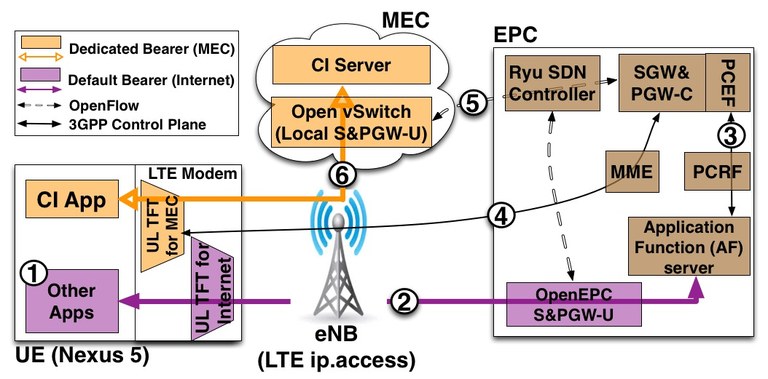
The figure above shows the detailed ACACIA Mobile Edge Network procedure.
-
Initially, the User Equipment (UE) is connected to the mobile network via a default bearer.
-
Send a MEC connectivity request from the CI app on the UE to the MEC Registration Server (MRS).
-
Create policy rules for the user’s CI app.
-
Setup a dedicated bearer in network for the user’s CI App through GW-Cs, MME, eNodeb and LTE modem in mobile device.
-
Setup flow rules in local S&PGW-U for the dedicated bearer.
-
The CI app interacts with CI server.
6. ACACIA Mobile Edge Network Protocol
This sequence diagram shows what protocols and messages are exchanged when you use ACACIA Mobile Edge Network. It is essentially the same as the procedure to trigger a dedicated bearer in LTE network.

The figures below show screenshots when we use the ACACIA profile. You can find all tcpdump files (you can find them /opt/acacia-gw/acacia-tcpdump/ directory in sgwu1 or pgwu1 node) which contains the control messages involved in this interaction.
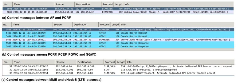
7. Limitation and Plan for ACACIA Mobile Edge Network
1. Short term plan
- The profile only supports one local SGWU and PGWU. We will extend the profile to support multiple local GWUs.
- After "bearer release" happens due to a radio idle timeout, the local SGW-U is not updated. So, it loses the dedicated bearer connection. We will support this function soon.
- Delete "dedicated bearer" connection on demand.
2. Long term plan
- You can specify your service name and its QCI value in a current profile. We plan to support more parameters for better traffic control for the service.

- Combine our extensions with Open Air Interface (OAI) to make all component public.
8. For questions or comments,
contact Junguk Cho <junguk.cho at utah.edu>
acacia-service-registration
This page shows how to add your own service. First, access OpenEPC web interface with your web browser ( epc.<your experiment name>.<your project name>.emulab.net )
It will ask id and passwd to login the page. We use admin for id and epc for passwd.
1. Click "PCC" -> "PCRF" -> "Policy Rules" -> "Search" buttons.

2. Add your service ( e.g., "ACACIA-AR" ) in "Name" blank and click "New" button.

3. Set "QCI" values from 6 to 9 and click "Update" button.

4. Click "PCC" -> "PCRF" -> "Policy Rulesets" -> "Search" buttons.

5. Click "OpenEPC Rel1 Test"

6. Select "ACACIA-AR" in List Of Rules and click "Add" button and "Update" button.

7. Now, you can use your own service in the profile
SIMECA: SDN-based IoT mobile edge cloud architecture
1. Tutorial Overview
This tutorial will show you how to initiate a SIMECA profile in PhantomNet and interact with SIMECA. At the end of the tutorial, you will have a sense of what SIMECA IoT mobile edge cloud is and how it works. You will be walked through experiments to (1) Attach a Nexus 5 device to SIMECA's core network and access a service in SIMECA's mobile edge cloud, (2) Attach an emulated User Equipment (UE) to SIMECA and set up a peer-to-peer connection between the emulated UE and the Nexus 5, (3) Perform a S1 seamless handover on the Nexus device while keeping an on-going peer-to-peer connection.
2. What is SIMECA?
SIMECA is a mobile core network that leverages SDN, NFV, and mobile edge cloud to provide low latency, low overhead for massive IoT devices. An overview of SIMECA is shown in figure 1: SIMECA architecture consists of three parts: SDN-enabled base stations (S-BS), SDN edge Network, and Edge Cloud. Here we will only provide an overview of SIMECA. If you are interested about the details, please refer to the paper.
- SDN-enabled base stations: are a set of base stations that are capable of SDN switch. The SDN-enabled base stations have OpenFlow interface to receive OpenFlow control messages from a SDN controllers (MCs) and install SDN rules in them. The S-BS classifies packets from the radio interface and passes them to the SDN edge network which delivers them to the server in the Edge Cloud. Applying SDN rules from an SDN controller, S-BS translates IP header of packets from User Equipment (UE) to a new IP header that is used by the SDN edge Network for forwarding.
- SDN edge Network: consists of multiple SDN switches that connects the S-BS to the Edge Cloud. The SDN switches forward UE's packets from the S-BS to the server that the UE is attached to. The SDN edge Network forwards packet using prefix matching on IP header.
- Edge Cloud: the edge cloud hosts both IoT services and NFV-based mobility functions. For example, Mobility Controller (MC) and Mobility Function (MF) are two component of the control plane of SIMECA are hosted in Edge Cloud. Using edge cloud, SIMECA reduces latency of both IoT services and SIMECA control plane. Also, the Edge Cloud allows flexibility and agility in deploying IoT services and SIMECA network functions.
- SIMECA Region: SIMECA consists of multiple regions each consists of three parts as above. The regions are interconnected by Gateway Switch. We envision a SIMECA region would correspond to a small metropolitan area with latency between S-BS and Edge Cloud is within several milliseconds.

Figure 1: SIMECA overview
SIMECA proposes a forwarding scheme at the S-BS and edge network and a routing scheme to:
- Eliminate GTP tunneling in mobile core network to provide a low overhead control plane for IoT.
- Reduce packet header in the mobile core to reduce data plane overhead for small packets generated by IoT devices.
- Enable Peer-to-peer communications for IoT devices.
- Support mobility and enable a low end-to-end latency for both IoT services and control plane.
Please refer the paper for more details.
3. SIMECA prototype in PhantomNet
We package a prototype of SIMECA as a profile in PhantomNet. The topology of this prototype is shown below:

Figure 2: SIMECA prototype in PhantomNet.
The prototype consists of:
- S-BS: the S-BS has three base stations - two emulated modified OpenEPC base stations and one modified OpenAirInterface SDR eNodeB running on USRP-B210 hardware. The radio link between Nexus 5 and the SDR base station is an RF link. Each base station has a default route to an Open Vswitch. The Open Vswitch (OVS) enables SDN functionality for the base station.
- Open Vswitch SDN Edge Network: there is a simple OVS to mimic an SDN edge network. The switch performs shortest path forwarding to forward packets between S-BS and Edge Cloud.
- Edge Cloud: there is one normal Ubuntu 12.04 server and an OVS attached to it in the Edge cloud.
- SIMECA control plane: The control plane of SIMECA ( MC and MF) is hosted on an node running Ubuntu 12.04 together with the modified MME.
4. Before you start
You need to obtain a permission to use a disk image in this experiment. Therefore you need to request the permission by sending an email to our support. Please follow this link.
5. Instantiate SIMECA prototype
To create your SIMECA prototype, instantiate an experiment using "simeca-sdr" profile:
"Actions" --> "Start Experiments" --> "Change Profile" --> search for "simeca-sdr" --> "Select Profile" --> "simeca-sdr"
More detailed information about how to instantiate an experiment using a profile, please see this.
6. SIMECA's source code:
The source code for SIMECA is in /opt/simeca. This includes implementation of MC, MF, and scripts to run SIMECA. The code for OpenEPC is hidden because of license permission. The code for OAI eNodeB is on the Penb1 node in /usr/local/src/airinterface/openairinterface5g.
You are welcome to modify SIMECA's controller code (/opt/simeca/simeca_controller/). Just copy the code to your home directory and modify it. The code is under Apache License (https://www.apache.org/licenses/LICENSE-2.0).
7. Initialize SIMECA
To run SIMECA, we first need to configure and run the OVSes in S-BS and SDN edge network as well as generate UE's subscription information in Home Subscriber Service (HSS) and a topology of the network with port information for shortest path forwarding module.
We have a start script that configs and set up all information to run SIMECA. Because the script also executes remote command on other nodes in the experiment (using ssh), you need to pass in your authentication information (using flag -YA in ssh) when log in to the SGW node to make this remote execution possible (otherwise you'll see the script asks for log in password which should not happen):
Log into SGW node: ssh -YA <your sgw node>
Important!! There is a script to initialize SIMECA. Before running the script, you need to change the UE's IMSI in the script so that the UE's information is populated into HSS database and the UE can attach to the network. To obtain UE's ID, in your experiment website click on List View to see the list of your nodes. For example, if your experiment is allocated UE7 (UE8), your UE_ID would be 306 (307). Feed in the UE_ID in the script on the SGW node:
On SGW node: sudo /opt/simeca/SCRIPTS/init_ue.sh
Now you can initialize SIMECA:
On SGW node (normal user): cd /opt/simeca/SCRIPTS; ./demo_init.sh
8. Start SIMECA controllers
We need to start SIMECA's control plane before doing other experiments. The SIMECA controllers consist of MF and MC that are running on a node named SGW. To start (or restart) them:
On SGW node (normal user): cd /opt/simeca/SCRIPTS; ./demo_restart.sh
When the script runs you will see the MME/emulated EnodeBs/MC/MF are restarted. At then end of the script, you'll see the MC is running and waiting for requests from MF (figure 3).

Figure 3. SIMECA controller started and is waiting for connection requests.
9. Scenario 1: Client-to-server connectivity
Step: Attach Nexus 5 to SIMECA's IoT core network.
In this first experiment we will see how SIMECA sets up a client-to-edge cloud server connection between a Nexus 5 and a server in the edge cloud. We'll need to run the OAI eNodeB by:
On Penb1 node: /usr/local/src/airinterface/openairinterface5g/SCRIPTS/run_lte_soft_modem.sh
The above script starts the OAI eNodeB. Once starts, the eNodeB will broadcast beacons and the Nexus 5 will automatically connect (figure 4). If the Nexus 5 does not try to attach to the eNodeB, try restart the Nexus 5. To restart the Nexus 5, log into adb-tgt node, and do:
On adb-tgt node: pnadb -a; adb reboot
After the Nexus 5 reboots and attaches to the eNodeB, you should see radio logs on the Penb1 as well as a note one the MC saying it installed a client-to-server path for the Nexus 5. The MC's log also shows the IP of the server that the Nexus 5 connected to and the Nexus 5's reachable IP address (figure 5).

Figure 4. Nexus 5 attached to the network successfully.

Figure 5. SIMECA controller shows it accepted a C2S connection from Nexus 5 (and the Nexus 5 device ID - IP address).
Step: Nexus 5 ping IoT server in edge cloud.
After the Nexus 5 connects to SIMECA, we can ping the server from Nexus 5. You should see around 15ms RTT from the Nexus 5 to the server. Notice that most of the latency comes from the radio latency.
On Adb-tgt node: pnadb -a; adb shell ping -c10 192.168.7.10
10. Scenario 2: Peer-to-peer connectivity
Step: Attach emulated UE to SIMECA.
To attach emulated UE to SIMECA, we need to trigger an Attach procedure on the emulated UE:
1. Log into client1 node via users.phantomnet.org: ssh -YA users.phantomnet.org
2. Attach to MM screen in client1: /opt/OpenEPC/bin/mm.attach.sh
3. (Inside the MM's screen) Trigger a network attach for the emulated UE: mm.connect_l3 LTE
Step: Peer-to-peer connection between Nexus 5 and emulated UE.
When the emulated UE attached, you should see that SIMECA sets up a peer-to-peer connection between the Nexus 5 and the emulated UE (the initialize script hardcoded in SIMECA configuration that SIMECA needs to set up this peer-to-peer connection always). In the UE's screen (mm screen), take note of the IP address the MC assigned to the emulated UE during attach (figure 6).

Figure 6. SIMECA's log showing a P2P connection between the Nexus 5 and the emulated UE was set up.
Once the emulated UE attached and the SIMECA controller finishes installing route, you can ping the emulated UE from the Nexus 5 (using the emulated UE's IP address in the UE's screen). You should see also around 13ms RTT.
On Adb-tgt node: adb shell ping <emulated UE's IP address (obtained in MC when the emulated UE attached).>
11. Scenario 3: Seamless handover
In this experiment we will let the emulated UE perform a seamless S1-handover while having an on-going connection with the Nexus 5. During the handover, you will see the emulated UE moves from eNodeb2 to eNodeb3 while the Ping session is not interrupted.
First, you need to start eNodeb3 which is the target eNodeB for the handover:
1. Log into enb3 node.
2. Start eNodeB: /opt/OpenEPC/bin/enodeb.start.sh
Second, while keeping the P2P Ping session in the last step, trigger a S1-handover on eNodeB2 by:
1. Log into enb2 node.
2. Attach to eNodeB's screen: /opt/OpenEPC/bin/enodeb.attach.sh
3. Perform S1-handover: enodeb.utah_intra_lte_handover 001011234567890 01 4569 192.168.3.32
The log on the emulated eNodeB will show that the emulated UE handed over from eNodeB2 to eNodeB3 (figure 7). While the handover happens, the Nexus 5 is still pinging the emulated UE just fine (without packet lost). This demonstrates seamless handover functionality in SIMECA.

Figure 7. EnodeB2's log showing S1-HO was performed successfully.
12. Conclusion
This tutorial walked you through the steps to instantiate a prototype of SIMECA using a prepackaged profile in PhantomNet. It show steps to repeat several experiments to demonstrate basic functionality of SIMECA: low latency client-to-server connectivity, low latency peer-to-peer connectivity, and seamless mobility. By walking you through the tutorial, we hope you had a better sense of what SIMECA is, how it works, and from that develop your own ideas of integrating SDN in mobile networks.
13. Acknowledgement
We develop our SDN-based base station based on OpenAirInterface SDR eNodeB implementation and Open Vswitch. Our emulated base station and MME are based on OpenEPC implementation. If you have questions please contact: binh@cs.utah.edu.
S1 handover with emulated UE and eNBs
Introduction
This tutorial shows how to use S1 handover with emulated UE and eNBs in PhantomNet. To get started, first instantiate an experiment with the Basic-OpenEPC profile via PhantomNet portal. When creating the experiment, increase the "Number of eNodeB nodes" to 2 or 3 (currently, 3 eNodeBs are maximum number of eNodeBs). In this tutorial, we assume your client is initially connected to enb1, and moves from enb1 to enb2. If you don't know how to perform the initial UE attachment with OpenEPC, please first go through the OpenEPC Tutorial. If your client is not connected to enb1 (e.g., enb2, enb3), you just need to change parameters in each command. S1 handover with emulated UE and eNBs needs some manual steps since emulated UE and eNBs in OpenEPC does not have radio procedures which needs S1 handover. However, the procedures among source, target eNB, MME, and SGW are the same as S1 handover standard.
Required information for S1 handover
For S1 handover, you need to know client imsi, enodeb's tac and cell id and ip address. Generally, your experiment has these values for them.
i) client imsi : 998980000001001
* Subsequent clients will increment from here. E.g., client2 would be 998980000001002
ii) eNBs information (you can check enodeb's tac and cell id information in /opt/OpenEPC/etc/enodeb.xml).
| cell id | ip address | TAC | |
| enb1 | 4567 | 192.168.3.29 | 01 |
| enb2 | 4568 | 192.168.3.30 | 01 |
| enb3 | 4569 | 192.168.3.31 | 01 |
iii) You can check which eNB is connected to UE for an initial connection for UE in enb's console.
# attach to enb's console
enb:~$ /opt/OpenEPC/bin/enodeb.attach.sh

# type "enodeb.print". With "help" command, you can see all possible commands.
eNodeB> enodeb.print
WARN:enodeb_console_print_sessions():82> IP address: [192.168.4.91]
WARN:execute_external():225> Sessions
Index: [7] IMSI: [998980000001001]
MME:[192.168.4.80|3550667]  ENB S1AP:[|7]
PDN Connection>  APN:[default]  Type:[1]
IPv4:[192.168.3.33/32]  IPv6:[]
ENB S1U:[192.168.4.91|7]
SGW S1U:[192.168.4.20|1717025697]
RAB> EBI:[5]
ENB S1U:[192.168.4.91|7]  SGW S1U:[192.168.4.20|1717025697]
Step 1: Trigger "Handover Request" in source eNB
i) ssh into the source enb (In this example, enb1)
ssh enb1.[your experiment name].[your project name].emulab.net
ii) attach to source enb's console
enb1:~$ /opt/OpenEPC/bin/enodeb.attach.sh
iii) type "handover request" in enb's console
# command format  enodeb.intra_lte_handover <imsi> <tac> <target enb's cell id>
eNodeB> enodeb.intra_lte_handover 998980000001001 01 4568
With this command, OpenEPC proceeds "Handover Command" procedure in S1 handover.
Step 2: Handover Notify in target eNB
i) ssh into the target enb (In this example, enb2)
ssh enb2.[your experiment name].[your project name].emulab.net
ii) attach to target enb's console
enb2:~$ /opt/OpenEPC/bin/enodeb.attach.sh
iii) type "handover request" in target enb's console
# command format  enodeb.handover_notify <imsi>
eNodeB> enodeb.handover_notify 998980000001001
With this command, OpenEPC executes the rest of S1 handover procedures.
Step 3: Set up routing table in UE
i) ssh into the ue
ii) change routing table
# command format
# sudo route add -net <target enb's ip> netmask 255.255.255.255 dev <client network interface which has "192.168.3.33">
# sudo route add default gw <target enb's ip> <client network interface which has "192.168.3.33">

client1:~$ sudo route add -net 192.168.3.30 netmask 255.255.255.255 dev eth5
client1:~$ sudo route add default gw 192.168.3.30 dev eth5
client1:~$ route -n
iii) send traffic from UE to Internet, which goes through target enb.
client1:~$ ping 8.8.8.8
Questions
For any other questions, contact phantomnet-users@emulab.net
S1 handover with emulated UE and eNBs and MME Relocation
Introduction
This tutorial shows how to use S1 handover with emulated UE and eNBs and MME Relocation in PhantomNet. To get started, first instantiate an experiment with the inter-mme-HO profile via PhantomNet portal. When creating the experiment, increase the "Number of eNodeB nodes" to 2 and "Node Hardware Type" to any available physical machine type. In this tutorial, your client is initially connected to enb1 and mme1, and moves from enb1&mme1 to enb2&mme2. If you don't know how to perform the initial UE attachment with OpenEPC, please first go through the OpenEPC Tutorial. S1 handover with emulated UE and eNBs and MME relocation needs some manual steps since emulated UE and eNBs in OpenEPC do not have the required RAN procedures for handover. However, the procedures among source, target eNBs and MMEs, and SGW are the same as S1 handover standard.
Prerequisite configurations for S1 handover with MME relocation
For S1 handover with MME relocation, you need to know client imsi, enodeb and MME information for S1 handover. This information is listed below.
i) client imsi : 998980000001001
ii) eNodeB information (you can check enodeb's tac and cell id information in /opt/OpenEPC/etc/enodeb.xml).
| cell id | ip address | TAC | |
| enb1 | 4567 | 192.168.3.29 | 01 |
| enb2 | 4568 | 192.168.3.30 | 02 |
iii) MMEs information (you can check mme information in /opt/OpenEPC/etc/mme.xml).
| MMEGI | MMEC | ip address | |
| mme1 | 123 | 45 | 192.168.4.80 |
| mme2 | 23 | 21 | 192.168.4.87 |
iv) Component naming
| Node name in this profile | EPC Components |
| SGW | MME1 & SGW |
| MME1 | MME2 |
iv) Files for EPC function configurations. You will need to download them for the next step (Configurations for testing S1 handover with MME relocation).
| File | Contents |
| mme-ip.sh | Set up MME2 IP addresses |
| get_interface_map.pl |
1. Used in mme-ip.sh to get net-d, net-b and mgmt interface. 2. Used to get net_c interface in eNB2. |
| interMME-ho-mme1.xml | MME1 xml configuration |
| interMME-ho-mme2.xml | MME2 xml configuration |
| interMME-ho-enb2.xml | eNB2 xml configuration |
Configurations for testing S1 handover with MME relocation
To test S1 handover with MME relocation, you need to set up information shown above in each node. In addition, there are limitations on OpenEPC implementation to test S1 handover with MME relocation. For example, first run eNB1 and MME1 without running eNB2 and MME2 and do an initial attachment from UE. So, you should follow below procedures to test it.
i) Kill `enodeb` process on ENB2 node
# stop running enb2
$ sudo /opt/OpenEPC/bin/enodeb.kill.sh
ii) Set up MME1 (e.g., MMEGI, MMEC, MME2 info) for S1 handover
# Replace a current mme.xml file with a new mme.xml (interMME-ho-mme1.xml) file
$ sudo /opt/OpenEPC/phantomnet/check_oepc_config.pl -i interMME-ho-mme1.xml mme.xml

# Restart mme
$ sudo /opt/OpenEPC/bin/mme.kill.sh
$ sudo /opt/OpenEPC/bin/mme.start.sh
iii) Re-start ENB1
# Re-start enb1
$ sudo /opt/OpenEPC/bin/enodeb.kill.sh
$ sudo /opt/OpenEPC/bin/enodeb.start.sh
iv) Start UE attachment in CLIENT1 node (via `users.phantomnet.org`)
# Access to client1 console
$ /opt/OpenEPC/bin/mm.attach.sh
# Trigger an attachment request.
console> mm.connect_l3 LTE
v) After UE attachments, you need to configure ENB2 and MME2. First set up ENB2.
# Change parameters in interMME-ho-enb2.xml
# 1. Get net_c (an-lte) interface
$  perl get_interface_map.pl
LAN -> IFACE -> IP -> MAC
mgmt -> eth2 -> 10.10.1.6 -> 000423b73ea6
net-d -> eth3 -> 10.10.4.4 -> 000423b73ea7
an-lte -> eth5 -> 10.10.5.2 -> 000423b74041

# 2. eth5 is used for net_c (an-lte) interface in this experiment (In your experiments, the output will be different).
$ vim interMME-ho-enb2.xml
# Replace "net_c" with "eth5"

# Replace a current enodeb.xml file with a new enodeb.xml (interMME-ho-enb2.xml) file
$ sudo /opt/OpenEPC/phantomnet/check_oepc_config.pl -i interMME-ho-enb2.xml enodeb.xml

# Re-start enb2
$ sudo /opt/OpenEPC/bin/enodeb.kill.sh
$ sudo /opt/OpenEPC/bin/enodeb.start.sh
vi) Set up MME2
# Set up IP address for a second MME since MME2 was defined as "ANY" roles in this profile . So it does not have correct IP addresses for net-d, net-b and mgmt.
# You need to put get_interface_map.pl and mme-ip.sh in the same directory.
$ bash mme-ip.sh

# Replace a current enodeb.xml file with a new mme.xml (interMME-ho-mme2.xml)file
$ sudo /opt/OpenEPC/phantomnet/check_oepc_config.pl -i interMME-ho-mme2.xml mme.xml

# Re-start mme2
$ sudo /opt/OpenEPC/bin/mme.kill.sh
$ sudo /opt/OpenEPC/bin/mme.start.sh
Check configurations for testing S1 handover with MME relocation
i) Check connectivity between eNodeBs and MMEs
# In mme1, attach to mme console.
$ /opt/OpenEPC/bin/mme.attach.sh

# Print out a connected eNB info
console> mme.enb.print
Current Index [2] Current MME ID [4985879]
eNodeB: [2] IP [192.168.4.90] TAC [1] eNB-ID [4567] Connected IDs:
[S1AP IDs: 7-4985879] -> [MME Index 2]

# In mme2, attach to mme console.
$ /opt/OpenEPC/bin/mme.attach.sh

# Print out a connected eNB info
console> mme.enb.print
Current Index [2] Current MME ID [4746911]
eNodeB: [2] IP [192.168.4.91] TAC [2] eNB-ID [4568] Connected IDs:
[S1AP IDs: 7-4746911] -> [MME Index 2]
[S1AP IDs: 0-4746911] -> [MME Index 2]
ii) Check MME configurations in MME's console. You need to check GUMMEI, Served TA, and TA MCC information from MME's console with the information listed in "Prerequisite configurations for S1 handover with MME relocation"
# In mme1, attach to mme console.
$ /opt/OpenEPC/bin/mme.attach.sh

# Print out MME configuration info
console> mme.config.print
S1ap Address: [192.168.4.80]
S11 Address: [192.168.4.80]
S6a Address: [192.168.254.80]
GUMMEI: [MCC:998] [MNC:98][GroupID:123][Code:45]
MME Name: [MME_1.OpenEPC]
Security: [Primary EIA:1] [Secondary EIA:1][Primary EEA:0][Secondary EEA:0]
Other: [Hash size:24] [Relative Capacity:255][Combined IMSI/EPS Attach]
Served TA: MCC [998] MNC [098] TAC [00001]
Served TA: MCC [998] MNC [098] TAC [00001]
TA MCC [998] MNC [098] TAC [00002] GID [00023] CODE [021] MME [192.168.4.87]
RA MCC [001] MNC [001] TAC [0012] SGSN [192.168.4.120]

# In mme2, attach to mme console.
$ /opt/OpenEPC/bin/mme.attach.sh
# Print out MME configuration info
console) mme.config.print
S1ap Address: [192.168.4.87]
S11 Address: [192.168.4.87]
S6a Address: [192.168.254.87]
GUMMEI: [MCC:998] [MNC:98][GroupID:23][Code:21]
MME Name: [MME_1.OpenEPC]
Security: [Primary EIA:1] [Secondary EIA:1][Primary EEA:0][Secondary EEA:0]
Other: [Hash size:24] [Relative Capacity:255][Combined IMSI/EPS Attach]
Served TA: MCC [998] MNC [098] TAC [00002]
Served TA: MCC [998] MNC [098] TAC [00002]
TA MCC [998] MNC [098] TAC [00001] GID [00123] CODE [045] MME [192.168.4.80]
RA MCC [001] MNC [001] TAC [0012] SGSN [192.168.4.120]
Step 1: Trigger "Handover Request" in source eNodeB
i) ssh into the source eNodeB (In this example, ENB1)
ssh enb1.[your experiment name].[your project name].emulab.net
ii) attach to source eNodeB's console
enb1:~$ /opt/OpenEPC/bin/enodeb.attach.sh
iii) type "handover request" in enodeb console
# command format  enodeb.intra_lte_handover <imsi> <tac> <target enb's cell id>
eNodeB> enodeb.intra_lte_handover 998980000001001 02 4568
With this command, OpenEPC proceeds with the "Handover Command" procedure in S1 handover.
Step 2: Handover Notify in target eNB
i) ssh into the target eNodeB (In this example, ENB2)
ssh enb2.[your experiment name].[your project name].emulab.net
ii) attach to target eNodeB's console (ENB2)
enb2:~$ /opt/OpenEPC/bin/enodeb.attach.sh
iii) type "handover request" in target eNodeB's console (ENB2)
# command format  enodeb.handover_notify <imsi>
eNodeB> enodeb.handover_notify 998980000001001
With this command, OpenEPC executes the rest of S1 handover procedures.
Step 3: Set up routing table in UE
i) ssh into the CLIENT1 UE
ii) change routing table
# command format
# sudo route add -net <target enb's ip> netmask 255.255.255.255 dev <client network interface which has "192.168.3.33">
# sudo route add default gw <target enb's ip> <client network interface which has "192.168.3.33">

client1:~$ sudo route add -net 192.168.3.30 netmask 255.255.255.255 dev eth5
client1:~$ sudo route add default gw 192.168.3.30 dev eth5
client1:~$ route -n
iii) send traffic from UE to Internet, which goes through target enb.
client1:~$ ping 8.8.8.8
Limitations
i) Even though all procedures are done and CLIENT1 UE can send traffic to the internet through ENB2, MME1 dies after the S1 handover completes. There are apparently OpenEPC implementation issues in the last S1HO procedure which cause the MME1 function to crash.
ii) In a future revision, we will demonstrate how to elide most of the manual steps (configurations for testing S1 handover with MME relocation) with pre/post-hooks scripts.
Questions
For any other questions, contact phantomnet-users@emulab.net